Multiple Linear Regression Review Outline Simple Linear Regression

Multiple Linear Regression Review

Outline • Simple Linear Regression • Multiple Regression • Understanding the Regression Output • Coefficient of Determination R 2 • Validating the Regression Model

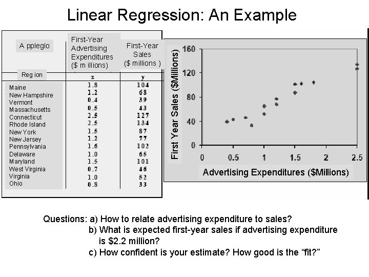
A ppleglo Reg ion Maine New Hampshire Vermont Massachusetts Connecticut Rhode Island New York New Jersey Pennsylvania Delaware Maryland West Virginia Ohio First-Year Advertising Expenditures ($ m illions) First-Year Sales ($ millions ) First Year Sales ($Millions) Linear Regression: An Example Advertising Expenditures ($Millions) Questions: a) How to relate advertising expenditure to sales? b) What is expected first-year sales if advertising expenditure is $2. 2 million? c) How confident is your estimate? How good is the “fit? ”

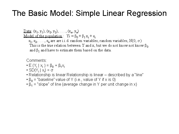
The Basic Model: Simple Linear Regression Data: (x 1, y 1), (x 2, y 2), . . . , (xn, yn) Model of the population : Yi = β 0 + β 1 xi + εi ε 1, ε 2, . . . , εn are i. i. d. random variables, N(0, σ ) This is the true relation between Y and x, but we do not know β 0 and β 1 and have to estimate them based on the data. Comments: • E (Yi | xi ) = β 0 + β 1 xi • SD(Yi | xi) = σ • Relationship is linear – described by a “line” • β 0 = “baseline” value of Y (i. e. , value of Y if x is 0) • β 1 = “slope” of line (average change in Y per unit change in x)

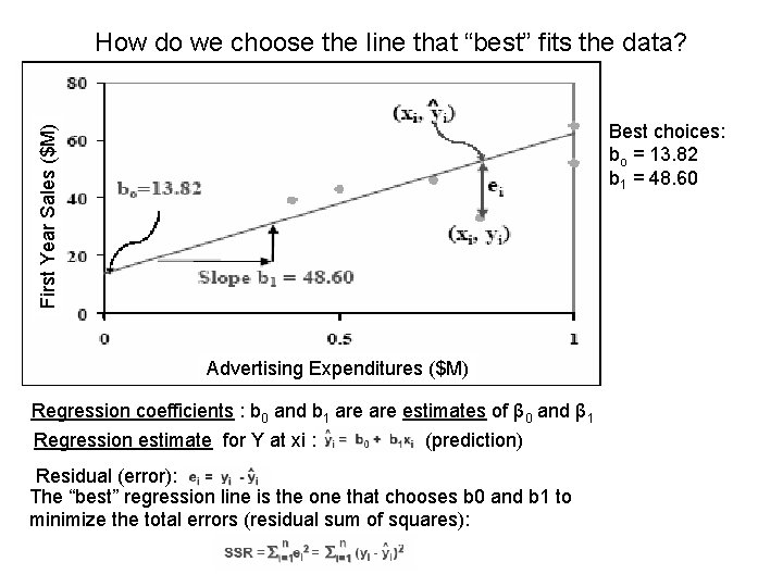
How do we choose the line that “best” fits the data? First Year Sales ($M) Best choices: bo = 13. 82 b 1 = 48. 60 Advertising Expenditures ($M) Regression coefficients : b 0 and b 1 are estimates of β 0 and β 1 Regression estimate for Y at xi : (prediction) Residual (error): The “best” regression line is the one that chooses b 0 and b 1 to minimize the total errors (residual sum of squares):

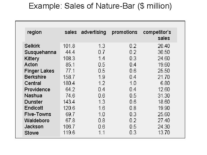
Example: Sales of Nature-Bar ($ million) region Selkirk Susquehanna Kittery Acton Finger Lakes Berkshire Central Providence Nashua Dunster Endicott Five-Towns Waldeboro Jackson Stowe sales advertising promotions competitor’s sales

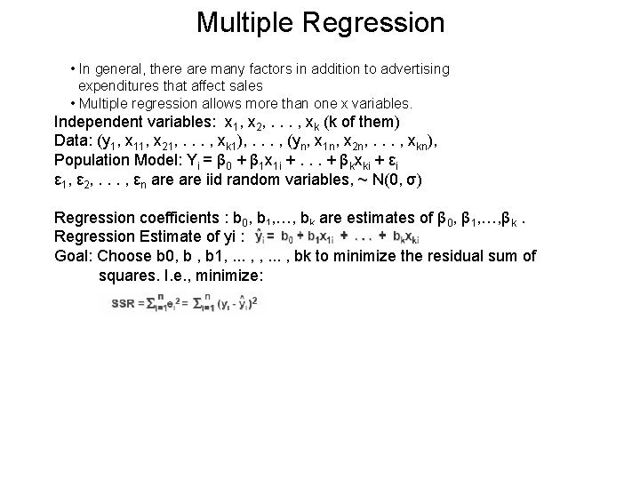
Multiple Regression • In general, there are many factors in addition to advertising expenditures that affect sales • Multiple regression allows more than one x variables. Independent variables: x 1, x 2, . . . , xk (k of them) Data: (y 1, x 11, x 21, . . . , xk 1), . . . , (yn, x 1 n, x 2 n, . . . , xkn), Population Model: Yi = β 0 + β 1 x 1 i +. . . + βkxki + εi ε 1, ε 2, . . . , εn are iid random variables, ~ N(0, σ) Regression coefficients : b 0, b 1, …, bk are estimates of β 0, β 1, …, βk. Regression Estimate of yi : Goal: Choose b 0, b 1, . . . , bk to minimize the residual sum of squares. I. e. , minimize:

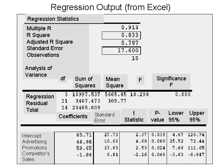
Regression Output (from Excel) Regression Statistics Multiple R R Square Adjusted R Square Standard Error Observations Analysis of Variance df Sum of Squares Regression Residual Total Coefficients Intercept Advertising Promotions Competitor’s Sales Mean Square Standard Error F t Statistic Significance F P- Lower value 95% Upper 95%

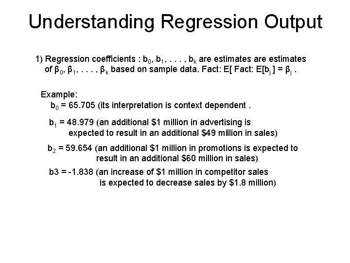
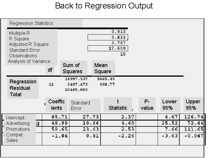
Understanding Regression Output 1) Regression coefficients : b 0, b 1, . . . , bk are estimates of β 0, β 1, . . . , βk based on sample data. Fact: E[bj ] = βj. Example: b 0 = 65. 705 (its interpretation is context dependent. b 1 = 48. 979 (an additional $1 million in advertising is expected to result in an additional $49 million in sales) b 2 = 59. 654 (an additional $1 million in promotions is expected to result in an additional $60 million in sales) b 3 = -1. 838 (an increase of $1 million in competitor sales is expected to decrease sales by $1. 8 million)

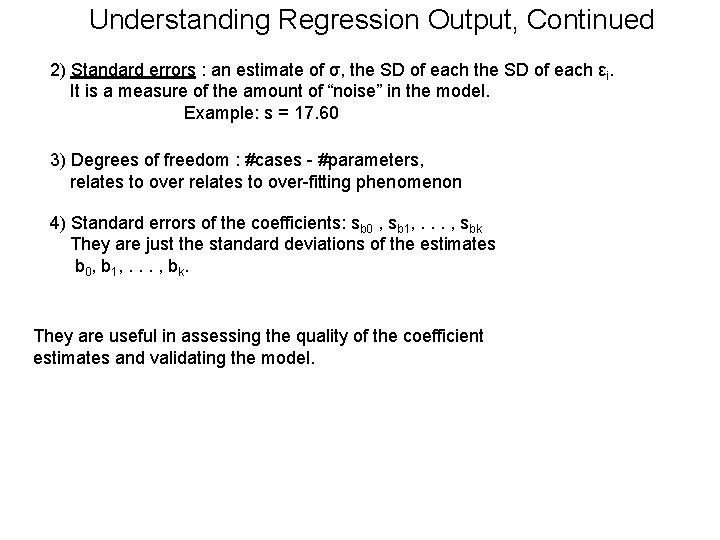
Understanding Regression Output, Continued 2) Standard errors : an estimate of σ, the SD of each εi. It is a measure of the amount of “noise” in the model. Example: s = 17. 60 3) Degrees of freedom : #cases - #parameters, relates to over-fitting phenomenon 4) Standard errors of the coefficients: sb 0 , sb 1, . . . , sbk They are just the standard deviations of the estimates b 0, b 1, . . . , b k. They are useful in assessing the quality of the coefficient estimates and validating the model.

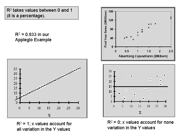
R 2 takes values between 0 and 1 (it is a percentage). R 2 = 0. 833 in our Appleglo Example R 2 = 1; x values account for all variation in the Y values R 2 = 0; x values account for none variation in the Y values

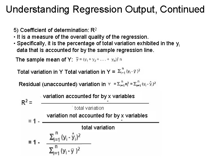
Understanding Regression Output, Continued 5) Coefficient of determination: R 2 • It is a measure of the overall quality of the regression. • Specifically, it is the percentage of total variation exhibited in the yi data that is accounted for by the sample regression line. The sample mean of Y: Total variation in Y = Residual (unaccounted) variation in Y variation accounted for by x variables total variation not accounted for by x variables total variation

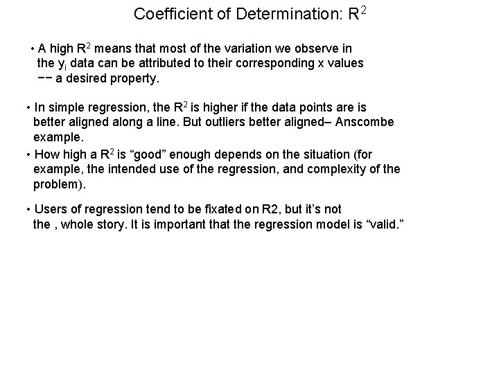
Coefficient of Determination: R 2 • A high R 2 means that most of the variation we observe in the yi data can be attributed to their corresponding x values −− a desired property. • In simple regression, the R 2 is higher if the data points are is better aligned along a line. But outliers better aligned– Anscombe example. • How high a R 2 is “good” enough depends on the situation (for example, the intended use of the regression, and complexity of the problem). • Users of regression tend to be fixated on R 2, but it’s not the , whole story. It is important that the regression model is “valid. ”

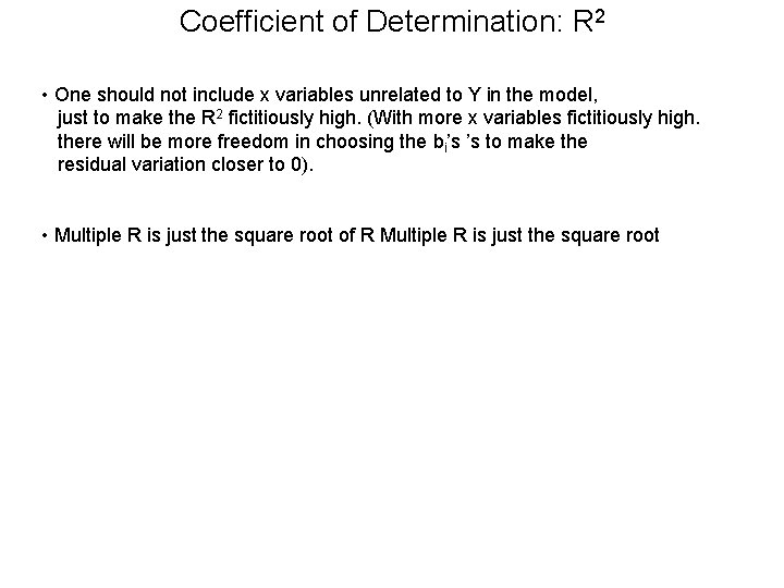
Coefficient of Determination: R 2 • One should not include x variables unrelated to Y in the model, just to make the R 2 fictitiously high. (With more x variables fictitiously high. there will be more freedom in choosing the bi’s ’s to make the residual variation closer to 0). • Multiple R is just the square root of R Multiple R is just the square root

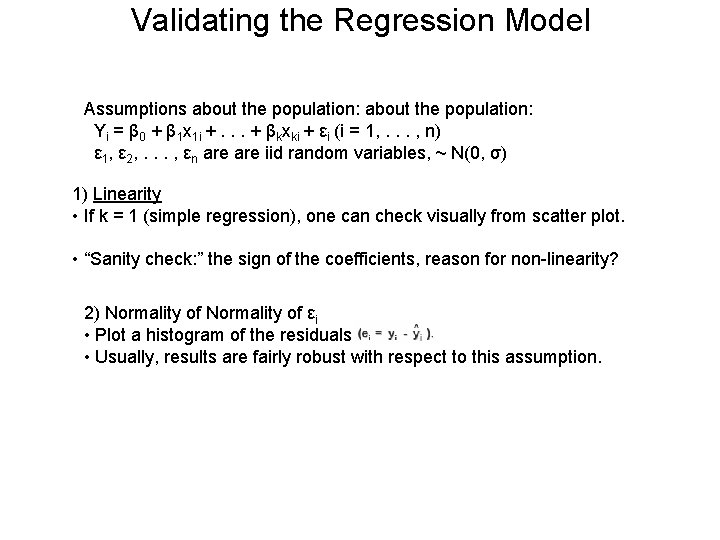
Validating the Regression Model Assumptions about the population: Yi = β 0 + β 1 x 1 i +. . . + βkxki + εi (i = 1, . . . , n) ε 1, ε 2, . . . , εn are iid random variables, ~ N(0, σ) 1) Linearity • If k = 1 (simple regression), one can check visually from scatter plot. • “Sanity check: ” the sign of the coefficients, reason for non-linearity? 2) Normality of εi • Plot a histogram of the residuals • Usually, results are fairly robust with respect to this assumption.

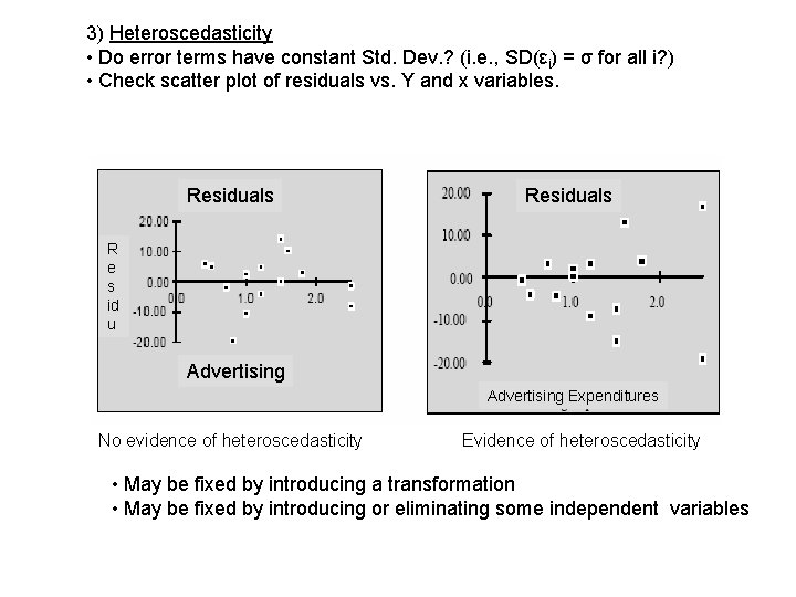
3) Heteroscedasticity • Do error terms have constant Std. Dev. ? (i. e. , SD(εi) = σ for all i? ) • Check scatter plot of residuals vs. Y and x variables. Residuals R e s id u Advertising Expenditures No evidence of heteroscedasticity Evidence of heteroscedasticity • May be fixed by introducing a transformation • May be fixed by introducing or eliminating some independent variables

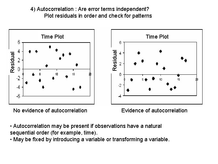
4) Autocorrelation : Are error terms independent? Plot residuals in order and check for patterns No evidence of autocorrelation Time Plot Residual Time Plot Evidence of autocorrelation • Autocorrelation may be present if observations have a natural sequential order (for example, time). • May be fixed by introducing a variable or transforming a variable.

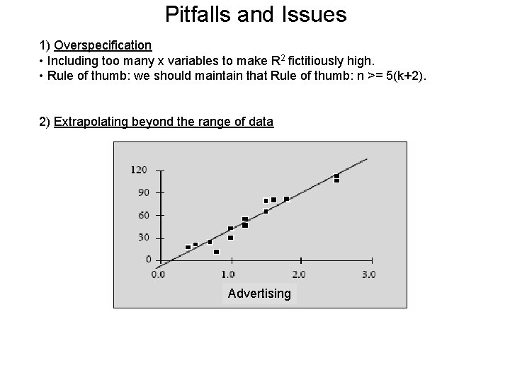
Pitfalls and Issues 1) Overspecification • Including too many x variables to make R 2 fictitiously high. • Rule of thumb: we should maintain that Rule of thumb: n >= 5(k+2). 2) Extrapolating beyond the range of data Advertising

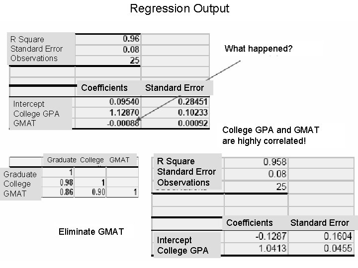
Validating the Regression Model 3) Multicollinearity • Occurs when two of the x variable are strongly correlated. • Can give very wrong estimates for βi’s. • Tell-tale signs: - Regression coefficients (bi’s) have the “wrong” sign. - Addition/deletion of an independent variable results in large changes of regression coefficients - Regression coefficients (bi’s ) not significantly different from 0 • May be fixed by deleting one or more independent variables

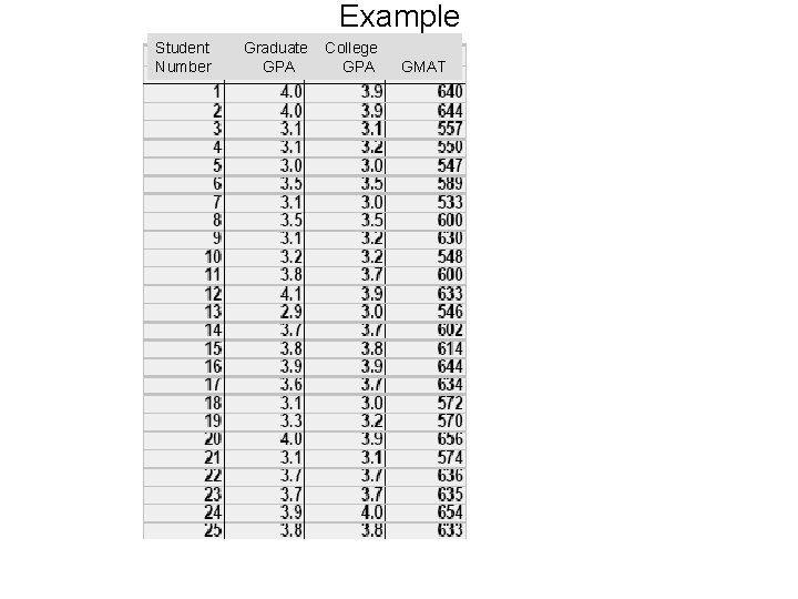
Example Student Number Graduate GPA College GPA GMAT

Regression Output R Square Standard Error Observations What happened? Coefficients Standard Error Intercept College GPA GMAT Graduate College GMAT Eliminate GMAT College GPA and GMAT are highly correlated! R Square Standard Error Observations Coefficients Intercept College GPA Standard Error

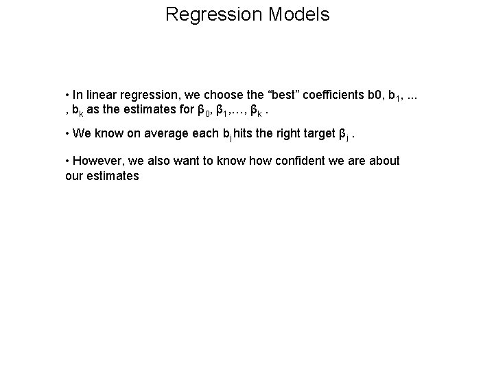
Regression Models • In linear regression, we choose the “best” coefficients b 0, b 1, . . . , bk as the estimates for β 0, β 1, …, βk. • We know on average each bj hits the right target βj. • However, we also want to know how confident we are about our estimates

Back to Regression Output Regression Statistics Multiple R R Square Adjusted R Square Standard Error Observations Analysis of Variance df Sum of Squares Mean Square Regression Residual Total Coeffic ients Intercept Advertising Promotions Compet. Sales Standard Error t Statistic Pvalue Lower 95% Upper 95%

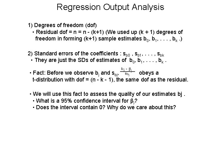
Regression Output Analysis 1) Degrees of freedom (dof) • Residual dof = n - (k+1) (We used up (k + 1) degrees of freedom in forming (k+1) sample estimates b 0, b 1, . . . , bk. ) 2) Standard errors of the coefficients : sb 0 , sb 1, . . . , sbk • They are just the SDs of estimates of b 0, b 1, . . . , bk. • Fact: Before we observe bj and sbj, obeys a t-distribution with dof = (n - k - 1), the same dof as the residual. • We will use this fact to assess the quality of our estimates bj. • What is a 95% confidence interval for βj? • Does the interval contain 0? Why do we care about this?

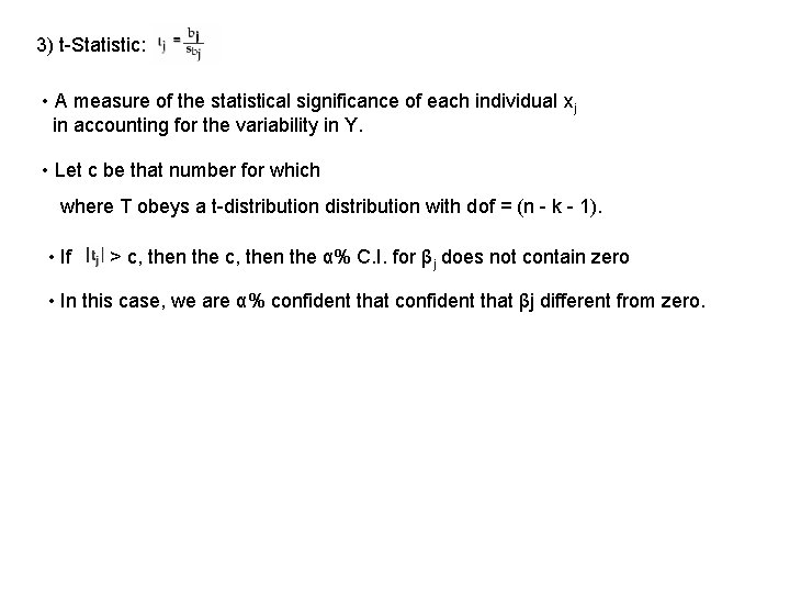
3) t-Statistic: • A measure of the statistical significance of each individual xj in accounting for the variability in Y. • Let c be that number for which where T obeys a t-distribution with dof = (n - k - 1). • If > c, then the α% C. I. for βj does not contain zero • In this case, we are α% confident that βj different from zero.

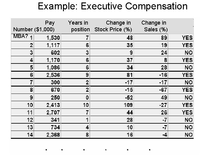
Example: Executive Compensation Pay Number ($1, 000) MBA? Years in Change in position Stock Price (%) Change in Sales (%)

variables: Dummy • Often, some of the explanatory variables in a regression are categorical rather than numeric. • If we think whether an executive has an MBA or not affects his/her pay, We create a dummy variable and let it be 1 if the executive has an MBA and 0 otherwise. • If we think season of the year is an important factor to determine sales, how do we create dummy variables? How many? • What is the problem with creating 4 dummy variables? • In general, if there are m categories an x variable can belong to, then we need to create m-1 dummy variables for it.

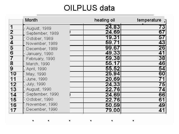
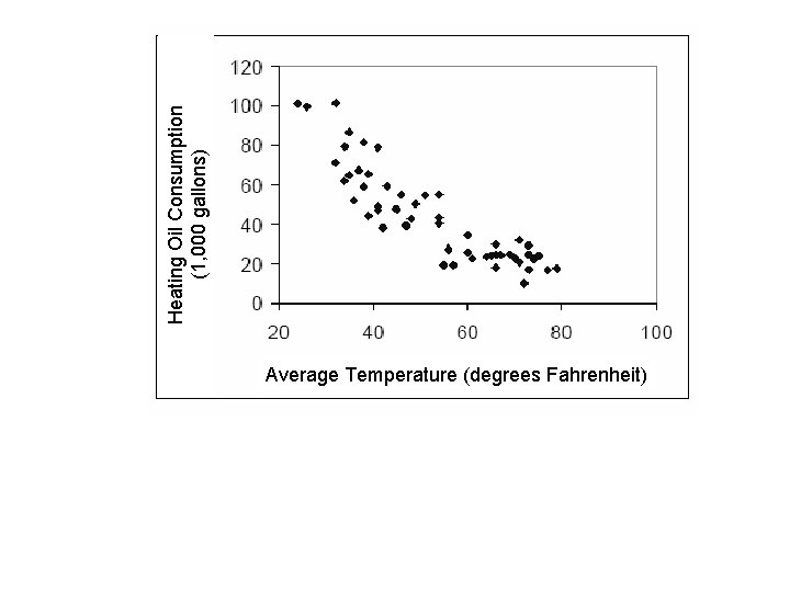
OILPLUS data Month August, 1989 September, 1989 October, 1989 November, 1989 December, 1989 January, 1990 February, 1990 March, 1990 April, 1990 May, 1990 June, 1990 July, 1990 August, 1990 September, 1990 October, 1990 November, 1990 December, 1990 heating oil temperature

Heating Oil Consumption (1, 000 gallons) Average Temperature (degrees Fahrenheit)

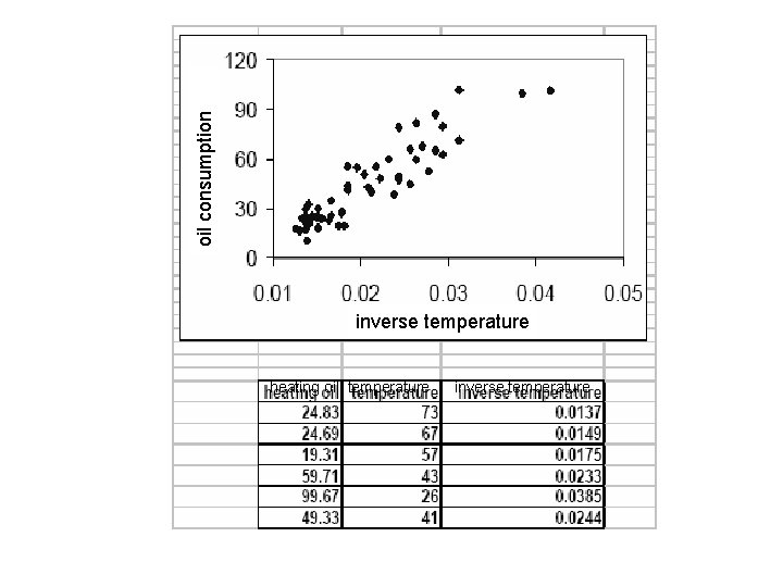
oil consumption inverse temperature heating oil temperature inverse temperature

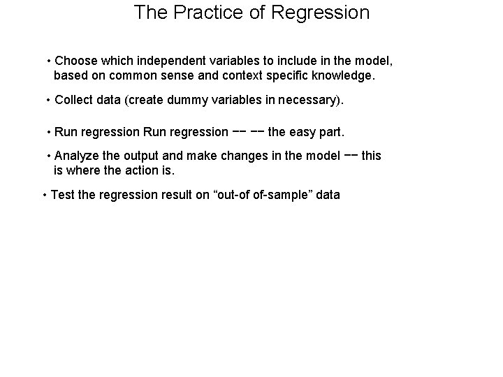
The Practice of Regression • Choose which independent variables to include in the model, based on common sense and context specific knowledge. • Collect data (create dummy variables in necessary). • Run regression −− −− the easy part. • Analyze the output and make changes in the model −− this is where the action is. • Test the regression result on “out-of of-sample” data

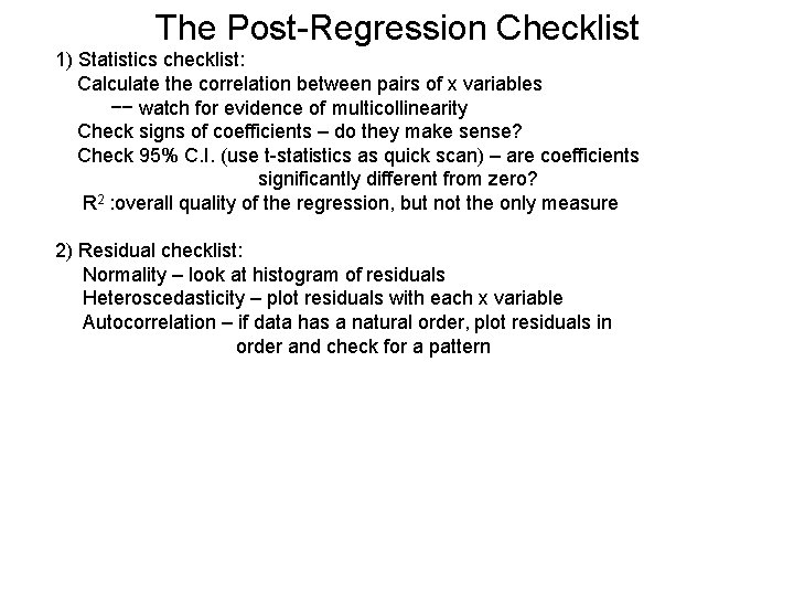
The Post-Regression Checklist 1) Statistics checklist: Calculate the correlation between pairs of x variables −− watch for evidence of multicollinearity Check signs of coefficients – do they make sense? Check 95% C. I. (use t-statistics as quick scan) – are coefficients significantly different from zero? R 2 : overall quality of the regression, but not the only measure 2) Residual checklist: Normality – look at histogram of residuals Heteroscedasticity – plot residuals with each x variable Autocorrelation – if data has a natural order, plot residuals in order and check for a pattern

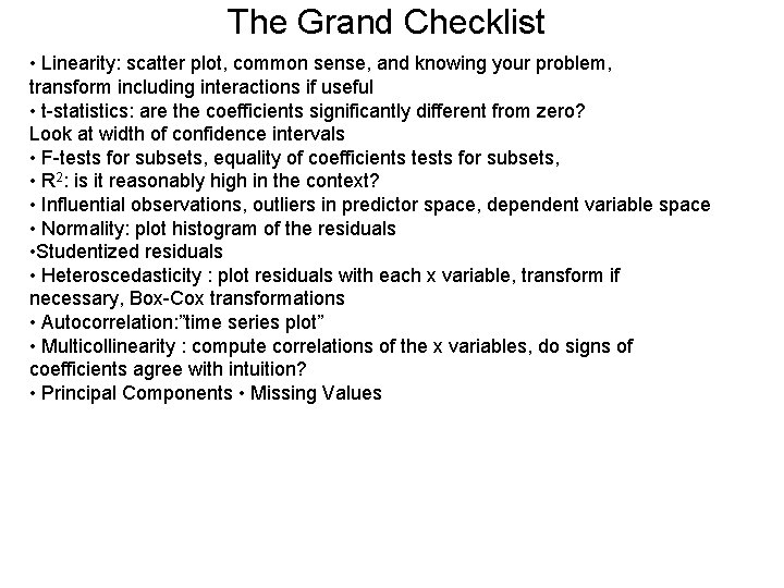
The Grand Checklist • Linearity: scatter plot, common sense, and knowing your problem, transform including interactions if useful • t-statistics: are the coefficients significantly different from zero? Look at width of confidence intervals • F-tests for subsets, equality of coefficients tests for subsets, • R 2: is it reasonably high in the context? • Influential observations, outliers in predictor space, dependent variable space • Normality: plot histogram of the residuals • Studentized residuals • Heteroscedasticity : plot residuals with each x variable, transform if necessary, Box-Cox transformations • Autocorrelation: ”time series plot” • Multicollinearity : compute correlations of the x variables, do signs of coefficients agree with intuition? • Principal Components • Missing Values