Linear Regression using R Sungsu Lim Applied Algorithm

Linear Regression using R Sungsu Lim Applied Algorithm Lab. KAIST 1/35

Regression • Regression analysis answers questions about the dependencies of a response variable on one or more predictors, • including prediction of future values of a response, discovering which predictors are important, and estimating the impact of changing a predictor or a treatment on the value of the response. • In linear regression, models of the unknown parameters are estimated from the data using linear functions. (Usually, the conditional mean of Y given the value of X) 2/35

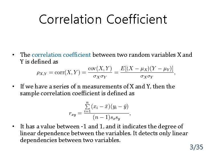
Correlation Coefficient • The correlation coefficient between two random variables X and Y is defined as • If we have a series of n measurements of X and Y, then the sample correlation coefficient is defined as • It has a value between -1 and 1, and it indicates the degree of linear dependence between the variables. It detects only linear dependencies between two variables. 3/35

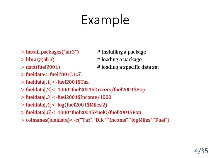
Example > install. packages("alr 3") # Installing a package > library(alr 3) # loading a package > data(fuel 2001) # loading a specific data set > fueldata<-fuel 2001[, 1: 5] > fueldata[, 1]<-fuel 2001$Tax > fueldata[, 2]<-1000*fuel 2001$Drivers/fuel 2001$Pop > fueldata[, 3]<-fuel 2001$Income/1000 > fueldata[, 4]<-log(fuel 2001$Miles, 2) > fueldata[, 5]<-1000*fuel 2001$Fuel. C/fuel 2001$Pop > colnames(fueldata)<-c("Tax", "Dlic", "Income", "log. Miles", "Fuel") 4/35

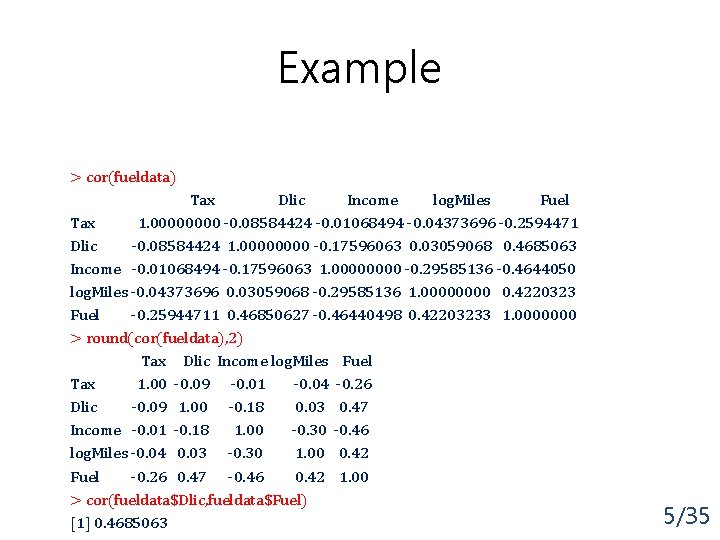
Example > cor(fueldata) Tax Dlic Income log. Miles Fuel Tax 1. 0000 -0. 08584424 -0. 01068494 -0. 04373696 -0. 2594471 Dlic -0. 08584424 1. 0000 -0. 17596063 0. 03059068 0. 4685063 Income -0. 01068494 -0. 17596063 1. 0000 -0. 29585136 -0. 4644050 log. Miles -0. 04373696 0. 03059068 -0. 29585136 1. 0000 0. 4220323 Fuel -0. 25944711 0. 46850627 -0. 46440498 0. 42203233 1. 0000000 > round(cor(fueldata), 2) Tax Dlic Income log. Miles Fuel Tax 1. 00 -0. 09 -0. 01 -0. 04 -0. 26 Dlic -0. 09 1. 00 -0. 18 0. 03 0. 47 Income -0. 01 -0. 18 1. 00 -0. 30 -0. 46 log. Miles -0. 04 0. 03 -0. 30 1. 00 0. 42 Fuel -0. 26 0. 47 -0. 46 0. 42 1. 00 > cor(fueldata$Dlic, fueldata$Fuel) [1] 0. 4685063 5/35

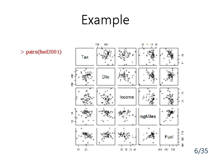
Example > pairs(fuel 2001) 6/35

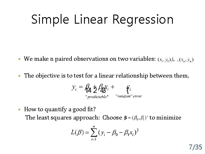
Simple Linear Regression • We make n paired observations on two variables: • The objective is to test for a linear relationship between them, • How to quantify a good fit? The least squares approach: Choose to minimize 7/35

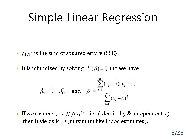
Simple Linear Regression • is the sum of squared errors (SSE). • It is minimized by solving , and we have and • If we assume i. i. d. (identically & independently) then it yields MLE (maximum likelihood estimates). 8/35

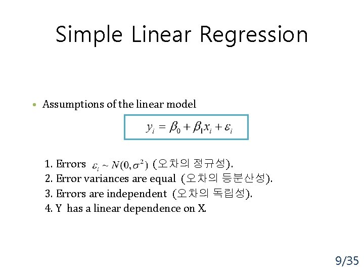
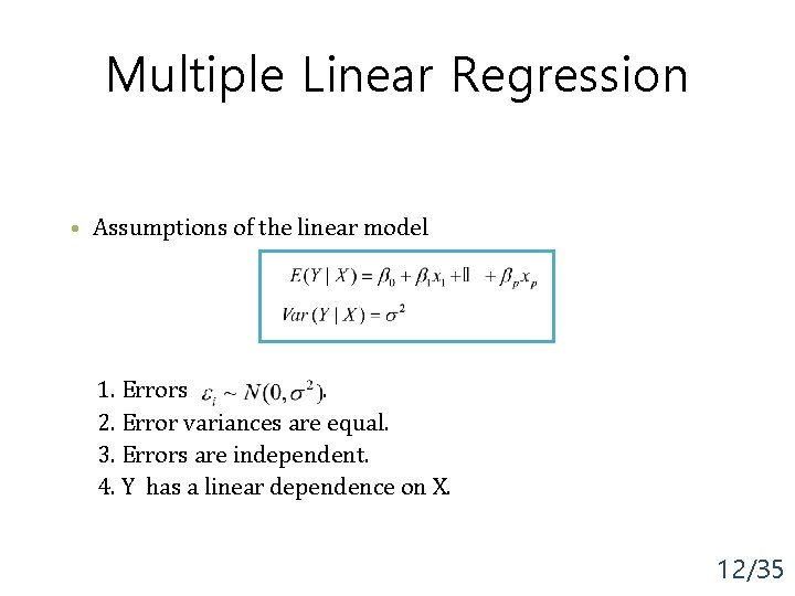
Simple Linear Regression • Assumptions of the linear model 1. Errors (오차의 정규성). 2. Error variances are equal (오차의 등분산성). 3. Errors are independent (오차의 독립성). 4. Y has a linear dependence on X. 9/35

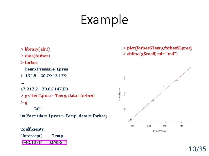
Example > library(alr 3) > data(forbes) > forbes Temp Pressure Lpres 1 194. 5 20. 79 131. 79 … 17 212. 2 30. 06 147. 80 > g<-lm(Lpres ~Temp, data=forbes) >g Call: lm(formula = Lpres ~ Temp, data = forbes) Coefficients: (Intercept) Temp -42. 1378 0. 8955 > plot(forbes$Temp, forbes$Lpres) > abline(g$coeff, col="red") 10/35

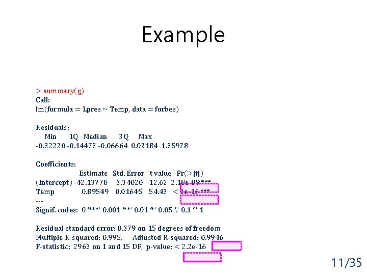
Example > summary(g) Call: lm(formula = Lpres ~ Temp, data = forbes) Residuals: Min 1 Q Median 3 Q Max -0. 32220 -0. 14473 -0. 06664 0. 02184 1. 35978 Coefficients: Estimate Std. Error t value Pr(>|t|) (Intercept) -42. 13778 3. 34020 -12. 62 2. 18 e-09 *** Temp 0. 89549 0. 01645 54. 43 < 2 e-16 *** --Signif. codes: 0 ‘***’ 0. 001 ‘**’ 0. 01 ‘*’ 0. 05 ‘. ’ 0. 1 ‘ ’ 1 Residual standard error: 0. 379 on 15 degrees of freedom Multiple R-squared: 0. 995, Adjusted R-squared: 0. 9946 F-statistic: 2963 on 1 and 15 DF, p-value: < 2. 2 e-16 11/35

Multiple Linear Regression • Assumptions of the linear model 1. Errors. 2. Error variances are equal. 3. Errors are independent. 4. Y has a linear dependence on X. 12/35

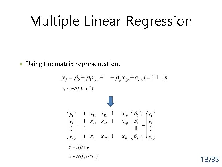
Multiple Linear Regression • Using the matrix representation, 13/35

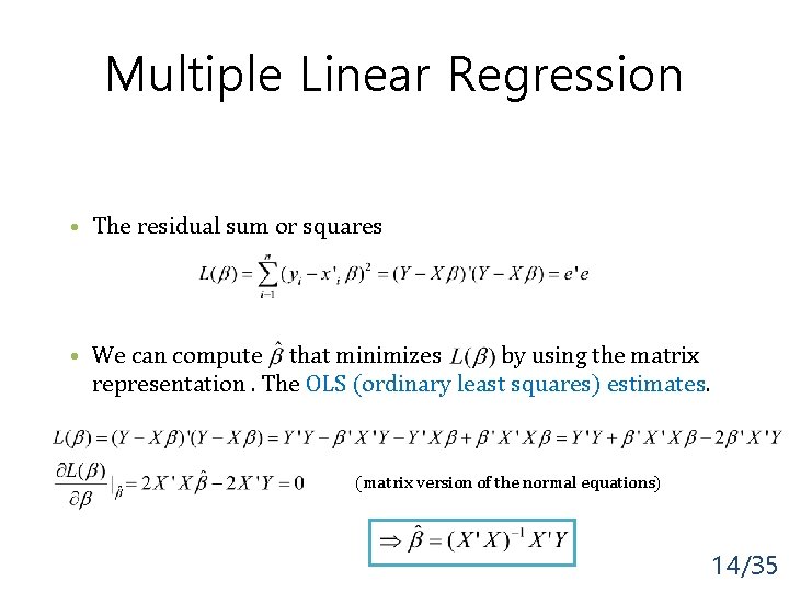
Multiple Linear Regression • The residual sum or squares • We can compute that minimizes by using the matrix representation. The OLS (ordinary least squares) estimates. (matrix version of the normal equations) 14/35

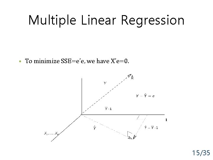
Multiple Linear Regression • To minimize SSE=e’e, we have X’e=0. 15/35

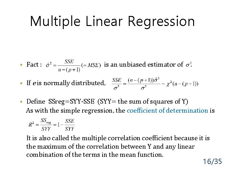
Multiple Linear Regression • Fact : is an unbiased estimator of . • If e is normally distributed, • Define SSreg=SYY-SSE (SYY= the sum of squares of Y) As with the simple regression, the coefficient of determination is It is also called the multiple correlation coefficient because it is the maximum of the correlation between Y and any linear combination of the terms in the mean function. 16/35

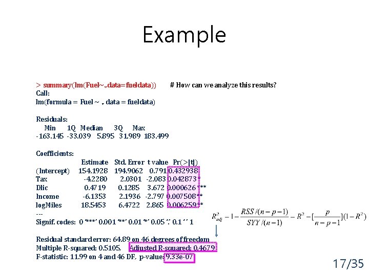
Example > summary(lm(Fuel~. , data=fueldata)) Call: lm(formula = Fuel ~. , data = fueldata) # How can we analyze this results? Residuals: Min 1 Q Median 3 Q Max -163. 145 -33. 039 5. 895 31. 989 183. 499 Coefficients: Estimate Std. Error t value Pr(>|t|) 154. 1928 194. 9062 0. 791 0. 432938 -4. 2280 2. 0301 -2. 083 0. 042873 * 0. 4719 0. 1285 3. 672 0. 000626 *** -6. 1353 2. 1936 -2. 797 0. 007508 ** 18. 5453 6. 4722 2. 865 0. 006259 ** (Intercept) Tax Dlic Income log. Miles --Signif. codes: 0 ‘***’ 0. 001 ‘**’ 0. 01 ‘*’ 0. 05 ‘. ’ 0. 1 ‘ ’ 1 Residual standard error: 64. 89 on 46 degrees of freedom Multiple R-squared: 0. 5105, Adjusted R-squared: 0. 4679 F-statistic: 11. 99 on 4 and 46 DF, p-value: 9. 33 e-07 17/35

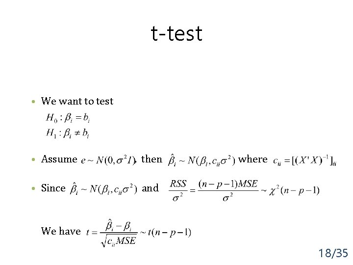
t-test • We want to test • Assume • Since , then where and We have 18/35

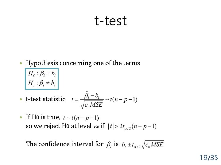
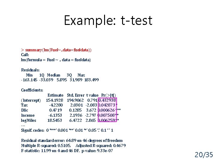
t-test • Hypothesis concerning one of the terms • t-test statistic: • If H 0 is true, , so we reject H 0 at level if The confidence interval for is 19/35

Example: t-test > summary(lm(Fuel~. , data=fueldata)) Call: lm(formula = Fuel ~. , data = fueldata) Residuals: Min 1 Q Median 3 Q Max -163. 145 -33. 039 5. 895 31. 989 183. 499 Coefficients: Estimate Std. Error t value Pr(>|t|) 154. 1928 194. 9062 0. 791 0. 432938 -4. 2280 2. 0301 -2. 083 0. 042873 * 0. 4719 0. 1285 3. 672 0. 000626 *** -6. 1353 2. 1936 -2. 797 0. 007508 ** 18. 5453 6. 4722 2. 865 0. 006259 ** (Intercept) Tax Dlic Income log. Miles --Signif. codes: 0 ‘***’ 0. 001 ‘**’ 0. 01 ‘*’ 0. 05 ‘. ’ 0. 1 ‘ ’ 1 Residual standard error: 64. 89 on 46 degrees of freedom Multiple R-squared: 0. 5105, Adjusted R-squared: 0. 4679 F-statistic: 11. 99 on 4 and 46 DF, p-value: 9. 33 e-07 20/35

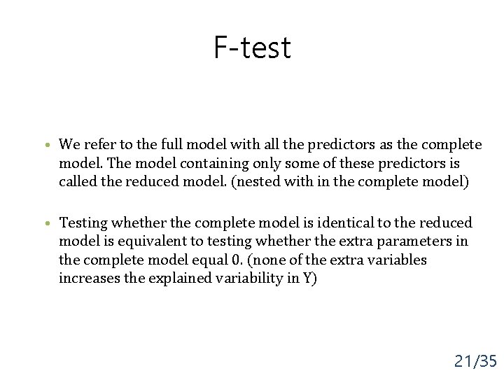
F-test • We refer to the full model with all the predictors as the complete model. The model containing only some of these predictors is called the reduced model. (nested with in the complete model) • Testing whether the complete model is identical to the reduced model is equivalent to testing whether the extra parameters in the complete model equal 0. (none of the extra variables increases the explained variability in Y) 21/35

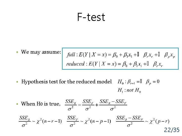
F-test • We may assume: • Hypothesis test for the reduced model • When H 0 is true, 22/35

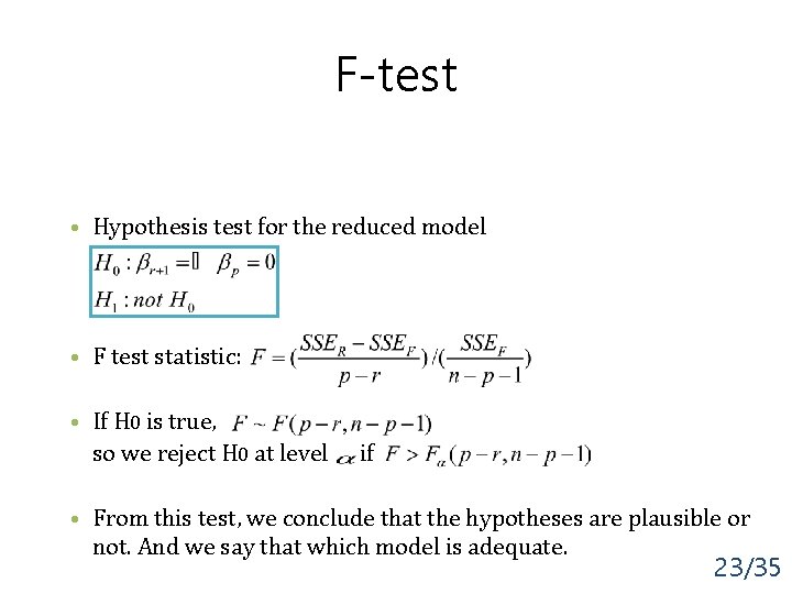
F-test • Hypothesis test for the reduced model • F test statistic: • If H 0 is true, so we reject H 0 at level if • From this test, we conclude that the hypotheses are plausible or not. And we say that which model is adequate. 23/35

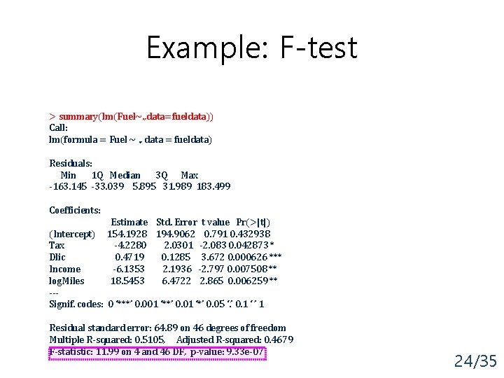
Example: F-test > summary(lm(Fuel~. , data=fueldata)) Call: lm(formula = Fuel ~. , data = fueldata) Residuals: Min 1 Q Median 3 Q Max -163. 145 -33. 039 5. 895 31. 989 183. 499 Coefficients: Estimate Std. Error t value Pr(>|t|) 154. 1928 194. 9062 0. 791 0. 432938 -4. 2280 2. 0301 -2. 083 0. 042873 * 0. 4719 0. 1285 3. 672 0. 000626 *** -6. 1353 2. 1936 -2. 797 0. 007508 ** 18. 5453 6. 4722 2. 865 0. 006259 ** (Intercept) Tax Dlic Income log. Miles --Signif. codes: 0 ‘***’ 0. 001 ‘**’ 0. 01 ‘*’ 0. 05 ‘. ’ 0. 1 ‘ ’ 1 Residual standard error: 64. 89 on 46 degrees of freedom Multiple R-squared: 0. 5105, Adjusted R-squared: 0. 4679 F-statistic: 11. 99 on 4 and 46 DF, p-value: 9. 33 e-07 24/35

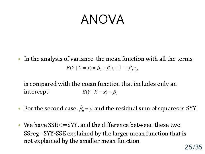
ANOVA • In the analysis of variance, the mean function with all the terms is compared with the mean function that includes only an intercept. • For the second case, and the residual sum of squares is SYY. • We have SSE<=SYY, and the difference between these two SSreg=SYY-SSE explained by the larger mean function that is not explained by the smaller mean function. 25/35

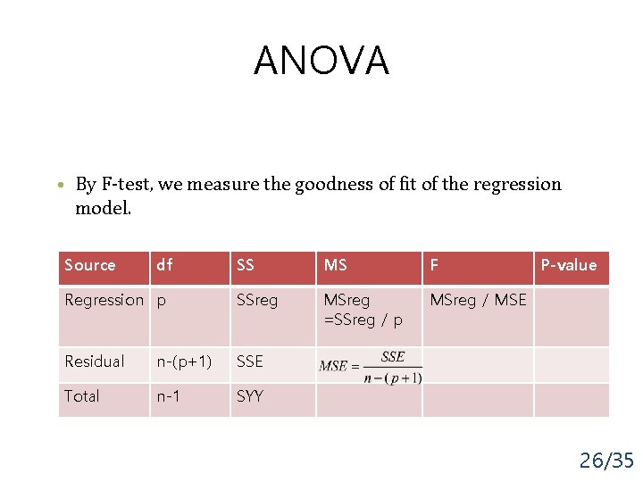
ANOVA • By F-test, we measure the goodness of fit of the regression model. Source df SS MS F Regression p SSreg MSreg =SSreg / p MSreg / MSE Residual n-(p+1) SSE Total n-1 SYY P-value 26/35

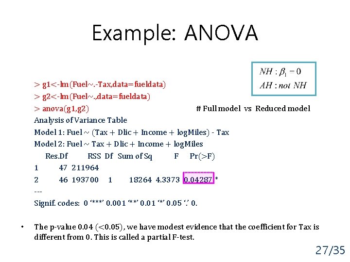
Example: ANOVA > g 1<-lm(Fuel~. -Tax, data=fueldata) > g 2<-lm(Fuel~. , data=fueldata) > anova(g 1, g 2) # Full model vs Reduced model Analysis of Variance Table Model 1: Fuel ~ (Tax + Dlic + Income + log. Miles) - Tax Model 2: Fuel ~ Tax + Dlic + Income + log. Miles Res. Df RSS Df Sum of Sq F Pr(>F) 1 47 211964 2 46 193700 1 18264 4. 3373 0. 04287 * --Signif. codes: 0 ‘***’ 0. 001 ‘**’ 0. 01 ‘*’ 0. 05 ‘. ’ 0. • The p-value 0. 04 (<0. 05), we have modest evidence that the coefficient for Tax is different from 0. This is called a partial F-test. 27/35

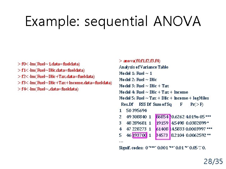
Example: sequential ANOVA > f 0<-lm(Fuel~1, data=fueldata) > f 1<-lm(Fuel~Dlic, data=fueldata) > f 2<-lm(Fuel~Dlic+Tax, data=fueldata) > f 3<-lm(Fuel~Dlic+Tax+Income, data=fueldata) > f 4<-lm(Fuel~. , data=fueldata) > anova(f 0, f 1, f 2, f 3, f 4) Analysis of Variance Table Model 1: Fuel ~ 1 Model 2: Fuel ~ Dlic Model 3: Fuel ~ Dlic + Tax Model 4: Fuel ~ Dlic + Tax + Income Model 5: Fuel ~ Tax + Dlic + Income + log. Miles Res. Df RSS Df Sum of Sq F Pr(>F) 1 50 395694 2 49 308840 1 86854 20. 6262 4. 019 e-05 *** 3 48 289681 1 19159 4. 5498 0. 0382899 * 4 47 228273 1 61408 14. 5833 0. 0003997 *** 5 46 193700 1 34573 8. 2104 0. 0062592 ** --Signif. codes: 0 ‘***’ 0. 001 ‘**’ 0. 01 ‘*’ 0. 05 ‘. ’ 0. 28/35

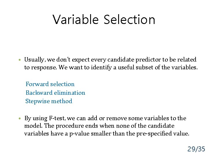
Variable Selection • Usually, we don’t expect every candidate predictor to be related to response. We want to identify a useful subset of the variables. Forward selection Backward elimination Stepwise method • By using F-test, we can add or remove some variables to the model. The procedure ends when none of the candidate variables have a p-value smaller than the pre-specified value. 29/35

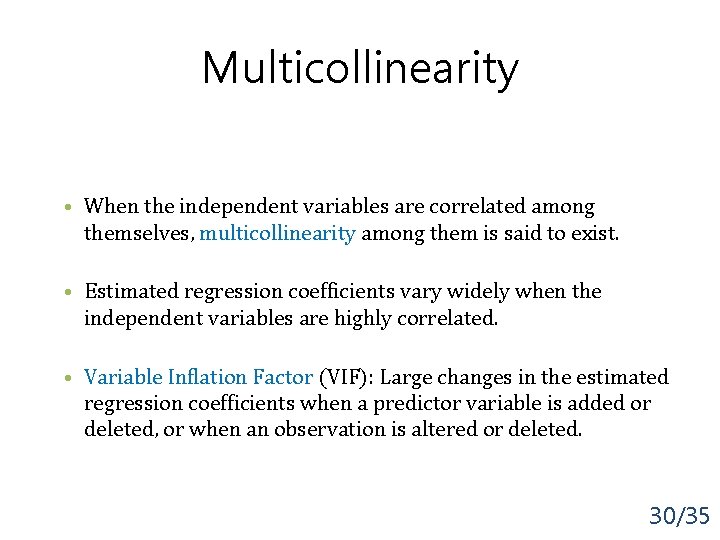
Multicollinearity • When the independent variables are correlated among themselves, multicollinearity among them is said to exist. • Estimated regression coefficients vary widely when the independent variables are highly correlated. • Variable Inflation Factor (VIF): Large changes in the estimated regression coefficients when a predictor variable is added or deleted, or when an observation is altered or deleted. 30/35

Multicollinearity • where is a coefficient of determination when is regressed on the other X variables. • VIFs measure how much the variances of the estimated regression coefficients are inflated as compared to when the predictor variables are not linearly related. • Generally, a maximum VIF value in excess of 5~10 is taken as an indication of multicollinearity. > vif(lm(Fuel~. , data=fueldata)) Tax Dlic Income log. Miles 1. 010786 1. 040992 1. 132311 1. 099395 31/35

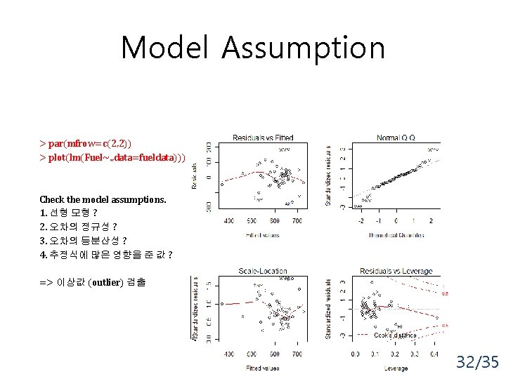
Model Assumption > par(mfrow=c(2, 2)) > plot(lm(Fuel~. , data=fueldata))) Check the model assumptions. 1. 선형 모형 ? 2. 오차의 정규성 ? 3. 오차의 등분산성 ? 4. 추정식에 많은 영향을 준 값 ? => 이상값 (outlier) 검출 32/35

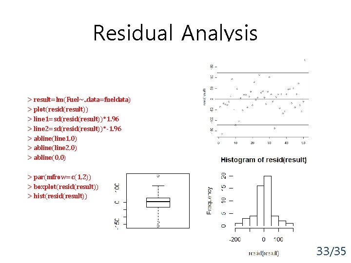
Residual Analysis > result=lm(Fuel~. , data=fueldata) > plot(resid(result)) > line 1=sd(resid(result))*1. 96 > line 2=sd(resid(result))*-1. 96 > abline(line 1, 0) > abline(line 2, 0) > abline(0, 0) > par(mfrow=c(1, 2)) > boxplot(resid(result)) > hist(resid(result)) 33/35

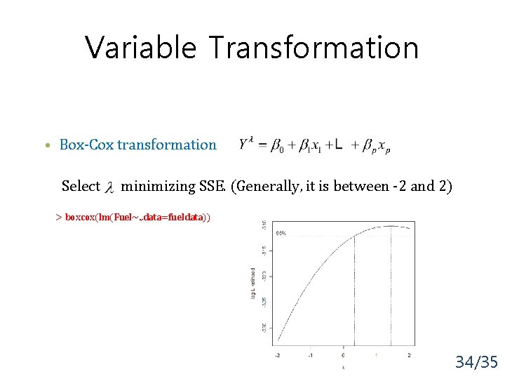
Variable Transformation • Box-Cox transformation Select minimizing SSE. (Generally, it is between -2 and 2) > boxcox(lm(Fuel~. , data=fueldata)) 34/35