Simple Linear Regression Review CORRELATION statistical technique used

Simple Linear Regression

Review CORRELATION: statistical technique used to describe the relationship between two interval or ratio variables Defined by r • Sign tells us direction of relationship (+ vs. -) • Value tells us consistency of relationship (-1 to +1) But what if we want to do more?

Regression = Prediction Let’s say Amherst declares war on Northampton because Northampton tries to lure Judie's into moving out of Amherst. We are all pacifists here in the Happy Valley, so we decide to settle our differences with a rousing game of Trivial Pursuit! You are elected the Captain of Amherst’s team (as if you would be selected instead of me). How are you going to choose the team? Multiple criteria: 1. Knowledge 2. Performance under pressure 3. Speed

Life Satisfaction Correlation: Do any of the following factors predict life satisfaction? – Money – Grades – Relationship status – Health Regression: If I know about your ____, (finances, GPA, relationships, health), I can predict your life satisfaction.

History - WWII We needed to place a ton of people into positions in which they would excel?

REGRESSION: statistical technique used to define the best fit equation that predicts the DV from one of more IV’s 5 4 Popularity Person A B C D E F G H I J K L M N Relational Aggression (x) Popularity (y) 5 4 5 5 3 5 4 4 4 5 4 2 4 3 3 4 3 2 2 1 1 1 3 1 2 3 2 1 0 0 1 2 3 Relational Aggression 4 5 Best fit line: identifies the central tendency of the relationship between the IV and the DV

The Regression Line Basics of linear equations Ŷ = 0 + 1 X …. . (or perhaps you know it as y = mx + b) Ŷ X 1 0 = predicted dependent variable (e. g. , popularity) = independent (predictor) variable (e. g. , relational aggression) = slope = y-intercept

Interpretation of y-intercept and slope Intercept ( 0) • Predicted value of Y when X is zero • Intercept only makes sense if X value can go down to zero. – e. g. heights (x) predicting weights (y) Slope ( 1) • Change in y for a one unit change in x. + implies direct relationship – implies inverse relationship

College GPA' = (0. 675)(High School GPA) + 1. 097 Ŷ = 0. 675 X + 1. 097 What would be the predicted GPA of someone with a 3. 0 high school GPA? College GPA' = (0. 675)(3. 0) + 1. 097 = 3. 122.

College GPA' = (0. 675)(High School GPA) + 1. 097 Ŷ = 0. 675 X + 1. 097 What would be the predicted GPA of someone with a 2. 0 high school GPA? College GPA' = (0. 675)(2. 0) + 1. 097 = 2. 447.

X X College GPA' = (0. 675)(High School GPA) + 1. 097 Ŷ = 0. 675 X + 1. 097 X College GPA' = (0. 675)(3. 0) + 1. 097 = 3. 122. X College GPA' = (0. 675)(2. 0) + 1. 097 = 2. 447 3. 122 – 2. 447=0. 675 (slope: change in Y for each 1 pt change in X)

How do we calculate a regression equation? Least-Squares method 1. Sum of the vertical distance between each Unbiased point and the line = 0. 1. Square of the vertical distance is as small as Minimum variability possible.

Calculating the slope and y-intercept Slope ( 1) = SP / SSx Intercept ( 0)= My – ( 1* Mx)

Leaving nothing to chance You’ve worked hard all semester long, but want to make sure you get the best possible grade. Would bribery help? Maybe. Let’s run a regression model to see if there is a relationship between monetary contributions to Jake and Abby’s College Fund and ‘Bonus Points for Special Contributions to Class’*. * Note: this is a humorous (? ) example, not an actual invitation to bribery.

Defining the regression line Subject Peeta Rue Katniss Thresh SSx SP X 4 8 2 6 x = 20 Y 1 9 5 5 y = 20 x 2 xy 16 4 64 72 4 10 36 30 (x 2) = 120 (xy) = 116 = = (x 2) – [( x)2 / n] 120 – [(20)2 / 4] 120 – (400 / 4) 120 – 100 = 20 = = (xy) – [ (x) y) / n] 116 – [(20) / 4] 116 – (400 /4) 116 – 100 = 16

Defining the regression line Subject Peeta Rue Katniss Thresh X 4 8 2 6 x = 20 Y 1 9 5 5 y = 20 x 2 Xy 16 4 64 72 4 10 36 30 (x 2) = 120 (xy) = 116 SSx= SP= 20 16 1 = = SP / SSx 16 / 20 = 0. 8 = = My – (b* Mx) 5 – (. 8)(5) = 1. 0 0

10 Rue 8 6 Katniss 4 Thresh 2 Peeta 0 0 2 4 6 Ŷ = 0. 8 x+1 8 10

Least Squares Method 1. Sum of the vertical distance between each point and the line = 0. 2. Square of the vertical distance is as small as possible.

Measuring Distance from the Regression Line (Error) Ŷ = 0. 8 x+1 10 9 Rue 8 7 6 Katniss 5 Thresh 4 3 2 1 Peeta 0 0 1 2 3 4 5 6 7 8 9

Measuring Error 10 Ŷ = 0. 8 x+1 Rue 8 6 Katniss 4 Thresh 2 Peeta 0 0 P R K T 2 4 x y 4 8 2 6 1 9 5 5 6 Ŷ = 0. 8 x+1 4. 2 7. 4 2. 6 5. 8 8 10 Distance (Y-Ŷ) -3. 2 1. 6 2. 4 -0. 8 ∑ = 0 Squared-Distance (Y-Ŷ) 2 10. 24 2. 56 5. 76 0. 64 ∑ (Y-Ŷ) 2 =19. 20

Standard error of the estimate •

x y 4 8 2 6 1 9 5 5 Ŷ = 0. 8 x+1 4. 2 7. 4 2. 6 5. 8 Distance Squared-Distance (Y-Ŷ) 2 1 – 4. 2 = -3. 2 10. 24 9 – 7. 4 = 1. 6 2. 56 5 – 2. 6 = 2. 4 5. 76 5 – 5. 8 = -0. 8 0. 64 ∑ =0 ∑ =19. 20 Standard Error of the Estimate “On Average, predicted scores differed from actual scores by 3. 1 points. ”

Standard Error and Correlation STE = 0 Small STE Large STE

Let it snow (3 x) I’m not a giant fan of winter, but I do kind of like sledding. I’m trying to convince a group of y’all to go sledding with me, but no one is interested. So, I buy a bunch of beer to try to convince you that sledding down Memorial Hill is a good idea. * I let you guys consume what you consider to be an appropriate amount of beer for a Tuesday night and then ask you to rate your interest in sledding on a 10 -point scale.

x (#drinks) 5 3 6 4 2 x = y (sledding) 10 6 7 3 4 y = x 2 y 2 xy 25 9 36 16 4 (x 2) = 100 36 49 9 16 (y 2) = 50 18 42 12 8 (xy) = 1. Find the regression equation 2. What is the predicted interest in sledding for someone who has consumed 2 drinks? 3. Calculate the standard error of the estimate (Y-

x (#drinks) 5 3 6 4 2 x = 20 SSx SP 1 0 = = y (sledding) 10 6 7 3 4 y = 30 x 2 y 2 xy 25 9 36 16 4 (x 2) = 90 100 36 49 9 16 (y 2) = 210 50 18 42 12 8 (xy) = 130 = (x 2) – [( x)2 / n] = (xy) – [ (x) y)] / n SP / SSx My – ( 1* Mx) (Y-

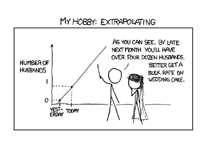
Using regression equations for prediction Ŷ = 1. 0(X) + 2 What do we expect Y to be if someone has 4 drinks Ŷ = 1. 0(X) + 2 = 1. 0(4)+2 = 6 BUT remember… 1. The predicted value is not perfect (unless the correlation between x and y = -1 or +1) 2. The equation cannot be used to make predictions about x values outside of the range of observed x values (e. g. Y when x is 20) 3. DO NOT confuse prediction with causation!

SSY Total Variability in Y SSregression Variability in Y explained by X Preview: this will be important for hypothesis testing in regression SSresidual Variability in Y NOT explained by X

Partitioning Variability in Y Squared correlation (r 2) tells us the proportion of variability in Y explained by X e. g. r 2 =. 65 means X explains 65% of the variability in Y SSregression = (r 2)SSY = (. 65)SSY

Partitioning Variability in Y Unpredicted variability will therefore = 1 - r 2 (variability not explained by x) e. g. if r 2 =. 65 then 35% of the variability in Y is not explained by x (1 -. 65=. 35) SSresidual = (1 -r 2)SSY = (. 35)SSY Alternative calculation of SSresidual = ∑(Y-Ŷ)2

x (#drinks) 5 3 6 4 2 x = 20 y (sledding) 10 6 7 3 4 y = 30 x 2 y 2 xy 25 9 36 16 4 (x 2) = 90 100 36 49 9 16 (y 2) = 210 50 18 42 12 8 (xy) = 130 SSx = 10 SP = 10 r 2 = . 582 = . 33 SSy=30 (Y 7 5 8 6 4 3 1 -1 -3 0 (Y= 20

x (#drinks) 5 3 6 4 2 x = 20 y (sledding) 10 6 7 3 4 y = 30 SSx = 10 x 2 y 2 xy 25 9 36 16 4 (x 2) = 90 100 36 49 9 16 (y 2) = 210 50 18 42 12 8 (xy) = 130 SP = 10 r 2 = . 582 = SSregression = (r 2)SSY = . 33 (30) SSresidual = (1 -r 2)SSY = 1 -. 33 (30) (Y 7 5 8 6 4 3 1 -1 -3 0 (Y= 20 SSy=30 = 9. 9 =. 67 (30) =20. 1

Hypothesis Testing for Regression If there is no real association between x and y in the population we expect the slope to equal zero If the slope for the regression line from our sample does not equal zero we must decide between two alternatives: 1. The nonzero slope is due to random chance error 2. The nonzero slope suggests a systematic real relationship between x and y that exists in the population

Null and Alternative for Regression Ho: the equation does not account for a significant proportion of the variance in the Y scores – Ho: b = 0 Ha: the equation does account for a significant proportion of the variance in Y scores. – Ha: b 0 Process of testing the regression line – Called analysis of regression – Very similar to ANOVA – F ratio used to determine if variance predicted is significantly greater than would be expected by chance

Calculating the F ratio • SSY SSregression SSresidual

Steps for Hypothesis Testing in Simple Regression Step 1: Specify the null and alternative hypotheses. – Ho: 1 = 0 – Ha: 1 0 Step 2: Designate the rejection region by selecting . Step 3: Obtain an F critical value df (1, n-2) Step 4: collect your data Step 5: Use your sample data to calculate the a) regression equation b) r 2 c) SS Step 6: Calculate the F ratio Step 7: Compare Fobs with Fcrit Step 8: Interpret results

Full Sledding Example x (#drinks) 5 3 6 4 2 x = 20 y (sledding) 10 6 7 3 4 y = 30 x 2 y 2 xy 25 9 36 16 4 (x 2) = 90 100 36 49 9 16 (y 2) = 210 50 18 42 12 8 (xy) = 130 (Y 7 5 8 6 4 Step 1: Specify the null and alternative hypotheses. – Ho: 1 = 0 – Ha: 1 0 Step 2: Designate the rejection region by selecting =. 05 Step 3: Obtain an F critical value df (1, n-2) = (1, 3) Fcrit = 10. 13 3 1 -1 -3 0 (Y= 20

Full Sledding Example x (#drinks) 5 3 6 4 2 x = 20 y (sledding) 10 6 7 3 4 y = 30 x 2 y 2 xy 25 9 36 16 4 (x 2) = 90 100 36 49 9 16 (y 2) = 210 50 18 42 12 8 (xy) = 130 Step 5: (a) calculate regression equation Ŷ = 1. 0 X + 2 (Y 7 5 8 6 4 Already Done! 3 1 -1 -3 0 (Y= 20

Full Sledding Example x (#drinks) 5 3 6 4 2 x = 20 y (sledding) 10 6 7 3 4 y = 30 Step 5: (b) Calculate r 2 = . 582 =. 33 x 2 y 2 xy 25 9 36 16 4 (x 2) = 90 100 36 49 9 16 (y 2) = 210 50 18 42 12 8 (xy) = 130 (Y 7 5 8 6 4 Already Done! 3 1 -1 -3 0 (Y= 20

Full Sledding Example x (#drinks) 5 3 6 4 2 x = 20 y (sledding) 10 6 7 3 4 y = 30 x 2 y 2 xy 25 9 36 16 4 (x 2) = 90 100 36 49 9 16 (y 2) = 210 50 18 42 12 8 (xy) = 130 (Y 7 5 8 6 4 Step 5: (c) Calculate SS SSregression = (r 2)SSY = 9. 9 SSresidual = (1 -r 2)SSY = 20. 1 Already Done! 3 1 -1 -3 0 (Y= 20

Full Sledding Example x (#drinks) 5 3 6 4 2 x = 20 y (sledding) 10 6 7 3 4 y = 30 x 2 y 2 xy 25 9 36 16 4 (x 2) = 90 100 36 49 9 16 (y 2) = 210 50 18 42 12 8 (xy) = 130 (Y 7 5 8 6 4 3 1 -1 -3 0 (Y= 20

Full Sledding Example x (#drinks) 5 3 6 4 2 x = 20 y (sledding) 10 6 7 3 4 y = 30 Step 6: Calculate F MSregression =9. 9 MSresidual =6. 7 x 2 y 2 xy 25 9 36 16 4 (x 2) = 90 100 36 49 9 16 (y 2) = 210 50 18 42 12 8 (xy) = 130 (Y 7 5 8 6 4 3 1 -1 -3 0 (Y= 20

Full Sledding Example x (#drinks) 5 3 6 4 2 x = 20 y (sledding) 10 6 7 3 4 y = 30 x 2 y 2 xy 25 9 36 16 4 (x 2) = 90 100 36 49 9 16 (y 2) = 210 50 18 42 12 8 (xy) = 130 (Y 7 5 8 6 4 3 1 -1 -3 0 (Y= 20 Step 7: Compare F obs to F crit Fcrit = 10. 13 Fobs = 1. 48 Decision: fail to reject the null Step 8: Interpretation: number of drinks does not account for a significant portion of the variance in attractiveness ratings

Summary Table SS Regression 9. 9 df 1 MS 9. 9 F 1. 48 Residual Total 3 4 6. 7 20. 1 30. 0 Number of drinks did not explain a significant proportion of the variance in willingness to go sledding with me, F(1, 3)=1. 48, p >. 05, R 2=. 33. Money down the toilet!!

Regression in RC Does weekend bedtime predict hours or TV viewing? Predictor (IV): Week end bed time Response (DV): hours of TV Step 1: Specify the null and alternative hypotheses. – Ho: 1 = 0 – Ha: 1 0 Step 2: Designate the rejection region by selecting =. 05 Step 3: Will judge significance using p-value method!

Regression in RC: WE bed & TV Coefficients: Estimate Std. Error t value Pr(>|t|) (Intercept) -5. 0234 2. 1189 -2. 371 0. 02487 * Week. End 0. 4291 0. 1523 2. 818 0. 00877 ** --Signif. codes: 0 '***' 0. 001 '**' 0. 01 '*' 0. 05 Residual standard error: 0. 7889 on 28 degrees of freedom Multiple R-squared: 0. 2209, Adjusted R-squared: 0. 1931 F-statistic: 7. 94 on 1 and 28 DF, p-value: 0. 00877

Regression in RC: WE bed & TV Coefficients: Estimate Std. Error t value Pr(>|t|) (Intercept) -5. 0234 2. 1189 -2. 371 0. 02487 * Week. End 0. 4291 0. 1523 2. 818 0. 00877 ** --Signif. codes: 0 '***' 0. 001 '**' 0. 01 '*' 0. 05 Residual standard error: 0. 7889 on 28 degrees of freedom Multiple R-squared: 0. 2209, Adjusted R-squared: 0. 1931 F-statistic: 7. 94 on 1 and 28 DF, p-value: 0. 00877

Writing up results of regression Weekend bedtime was a significant predictor of television viewing, F (1, 28) = 7. 94, p =. 01, r 2 = . 2209. The r 2 indicates that weekend bedtime explains 22. 09% of the variance in TV viewing. The slope of the regression equation was not significant (β 1 = 0. 4291, p =. 01) and indicated that people who went to sleep later tended to watch more TV (shame!). The regression equation relating weekend bedtime and TV viewing was: TV = -5. 0234 +. 4291(WE).

Standardized Slopes Standardized regression coefficient (β “beta”): standardized slope representing change of x and y in standard deviation units. Example: Ŷ = βx + a Ŷ =. 5 x + 10 • Interpretation of β: for each one SD increase in X there will be a corresponding. 5 SD increase in Y Why would we want a standardized coefficient? 1. Gives us a measure of effect size 2. If we have more than one predictor we can compare relative effects on Y

How do we calculate Beta? By Hand: 1. Transform Y scores into z scores 2. Transform X scores into z scores 3. Compute slope using transformed scores (then change will be in standard deviation units) (I won’t make you do this by hand!)

Real data examples

-What is R 2? -What is the standardized slope? -What does the standardized slope suggest about change in X vs. Y?

-Is self-esteem more strongly related to positivity or to negativity? -Calculate and interpret R 2 for the association between self-esteem and positivity