Chapter 10 Simple Linear Regression Simple Linear Regression

Chapter 10 Simple Linear Regression

Simple Linear Regression Chapter 10 introduces inference about a response variable from an explanatory variable. It is possible to perform this same type of analysis with multiple explanatory variables which you will see in Chapter 11 in MGT 310. Rather than break down this Chapter into sections I will break down the Chapter into steps to perfrom a simple linear regression.

TWO Quantitative Variables • When you have two quantitative variables often you would like to know if how these two variables are related or associated. • If you determine that the two quantitative variables are linearly associated it is appropriate to fit a line to the data. • Once a line has been fit you can then plug in any value of the explanatory variable to predict what the response variable will be.

For Example: A nation job placement company is interested in developing a model that might be used to explain the variation in starting salaries for college graduates based on the college GPA. The following data were collected through a random sample of the clients with which this company has been associated. GPA 3. 20 3. 40 2. 90 3. 60 2. 80 2. 50 3. 00 3. 60 2. 90 3. 50 Starting Salary $35, 000 $29, 500 $30, 000 $36, 400 $31, 500 $29, 000 $33, 200 $37, 600 $32, 000 $36, 000

Other Examples Example: College GPA and high school GPA Example: Test 3 Score and Test 4 Score Example: Mother’s heights and daughter’s heights

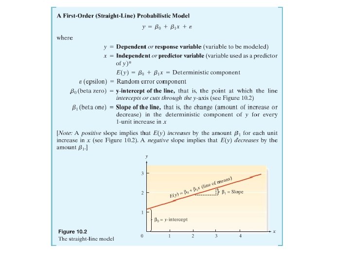
Before we begin looking a simple linear regression let’s review from your previous math courses what the equation for a line looks like. Recall: Where m is the slope and b is the y-intercept The concept covered in this Chapter fits a line to data with one response and one explanatory variable, then uses hypothesis testing to determine if the fit line can be used to predict values of the response variable.

Step-by-Step Process

EXAMPLE: For simplicity purposes we are going to use an example without any units x 3 1 3 5 y 5 8 6 4

Step 1: Hypothesize the deterministic component of the model that relates the mean E(y), to the independent variable x. We are considering only straight lines with one explanatory variable therefore the model in this Chapter will always be…

Step 2: Use the sample data to estimate unknown parameters in the model 1. Plot the data to a scattergram (or scatterplot) Determine whether fitting a line to the data seems appropriate based on the graph. (Note: not all data points will fall EXACTLY on line – it is an approximation)

Step 2: Use the sample data to estimate unknown parameters in the model Errors of prediction (ε) – deviations from the fitted prediction line 9 8 7 6 Y 5 4 3 2 1 0 0 1 2 3 X 4 5 6 GOAL: To fit a line that minimizes the errors of prediction

Step 2: Use the sample data to estimate unknown parameters in the model The line that minimizes these errors is called: • Least squares line • Least squares regression line • Regression line • Least square prediction line The methodology used to obtain this line is called the method of least squares.

Step 2: Use the sample data to estimate unknown parameters in the model Recall – We are finding the EQUATION for the line that best fits the sample data (to estimate the line for the population)

Step 2: Use the sample data to estimate unknown parameters in the model xx yy 33 55 0 -0. 75 0 0 15 9 25 11 88 -2 2. 25 -4. 5 4 8 1 64 33 66 0 0. 25 0 0 18 9 36 55 44 2 -1. 75 -3. 5 4 20 25 16 12 23 0 0 -8 8 61 44 141

Step 2: Use the sample data to estimate unknown parameters in the model x 3 1 3 5 12 y 5 15 8 8 6 18 4 20 23 61 9 25 44 25 64 36 16 141

Step 2: Use the sample data to estimate unknown parameters in the model 4. Be able to interpret these values y-intercept: the line crosses the y-axis at 8. 75 Slope: For every 1 unit increase in x there is a 1 unit decrease in y

Step 3: Specify the probability distribution of the random error term and estimate the standard deviation of this distribution Know the assumptions needed for the probability distribution of the random error ε Assumption 1: The mean of the probability distribution of ε is 0 – that is, the average of the values of ε over an infinitely long series of experiments is 0 for each setting of the independent variable x. This assumption implies that the mean value of y, E(y), for a given value of x is

Step 3: Specify the probability distribution of the random error term and estimate the standard deviation of this distribution Know the assumptions needed for the probability distribution of the random error ε Assumption 2: The variance of the probability distribution of ε is constant for all setting of the independent variable x. For our straight line model, this assumption means that the variance of ε is equal to a constant, say σ2, for all values of x. (We will estimate this by s 2)

Step 3: Specify the probability distribution of the random error term and estimate the standard deviation of this distribution Know the assumptions needed for the probability distribution of the random error ε Assumption 3: The probability distribution of ε is normal.

Step 3: Specify the probability distribution of the random error term and estimate the standard deviation of this distribution Know the assumptions needed for the probability distribution of the random error ε Assumption 4: The values of ε associated with any two observed values of y are independent – that is, the value of ε associated with one value of y has no effect on the values of ε associated with other y values.

Step 3: Specify the probability distribution of the random error term and estimate the standard deviation of this distribution Recall Assumption 3 – that ε’s have a constant variance – know how to estimate this value with s 2 (variability of random error term)

Step 3: Specify the probability distribution of the random error term and estimate the standard deviation of this distribution x 3 1 3 5 12 y 5 15 8 8 6 18 4 20 23 61 9 25 44 25 64 36 16 141

Step 3: Specify the probability distribution of the random error term and estimate the standard deviation of this distribution Be able to interpret this estimation of the standard deviation of the random error (in context of the problem)

Step 4: Assess Model Adequacy

Step 4: Assess Model Adequacy Hypotheses: One Tailed Test: Two Tailed Test:

Step 4: Assess Model Adequacy Assumptions: (same for assumptions as Step 3) 1. 2. 3. 4. ε’s have mean of 0 ε’s have constant variance ε’s are normally distributed ε’s are independent

Step 4: Assess Model Adequacy Test Statistic:

Step 4: Assess Model Adequacy Rejection Region: One-tailed: t<-tα when (or t>tα when ) Two-tailed: |t| > tα/2 tα and tα/2 based on (n-2) degrees of freedom

Step 4: Assess Model Adequacy Summary: If test statistic falls in rejection region OR p-value < α At the ___% significance level, my test statistic (t = ___) falls in the rejection region (or my p-value (_____) < α) therefore, I reject my null hypothesis. The data provides sufficient evidence to support that the slope of the line is (greater than, less than or different from) 0. If test statistic does not fall in rejection region OR p-value > α At the ___% significance level, my test statistic (t = ___) does not fall in the rejection region (or my p-value (______) > α) therefore, I do not reject my null hypothesis. The data provides insufficient evidence to support that the slope of the line is (greater than, less than or different from) 0.

Perform a two-tailed Hypothesis test for slope (using α = 0. 05) H 0: β 1 = 0 HA: β 1 ≠ 0 Where β 1 is the slope of the least squares regression equation for the population of x and y Assumptions 1. ε’s have a mean of 0 2. ε’s have constant variance 3. ε’s are normally distributed 4. ε’s are independent Test Statistic: Rejection Region:

At the 5% significance level the test statistic (t = -4. 619) falls in the rejection region therefore, I reject the null hypothesis. There is sufficient evidence to support the slope of the population data is different from 0.

Step 4: Assess Model Adequacy Calculate coefficient of correlation (r) x 3 1 3 5 12 y 5 15 8 8 6 18 4 20 23 61 9 25 44 25 64 36 16 141

Step 4: Assess Model Adequacy Interpret coefficient of correlation There is a strong negative linear relationship between x and y

Step 4: Assess Model Adequacy Calculate coefficient of determination (r 2)

Step 4: Assess Model Adequacy Interpret coefficient of determination (r 2)

Step 4: Assess Model Adequacy Interpret coefficient of determination (r 2) About 91. 43% of the variation in the sample of y can be explained by using x to predict y in our model

Step 5: When satisfied that model is useful, use it for prediction, estimation, and other purposes. How do we know model is useful? Statistically Useful if: Reject H 0 in hypothesis test for slope Practically Useful if: • 2 s is “small” (relative to values of y) • r 2 is “large”

Step 5: When satisfied that model is useful, use it for prediction, estimation, and other purposes. Use line for prediction and estimation Plug in value of x into equation to predict y at that level (Note: it is only appropriate to plug in value that are x-values used in the scope of the problem) Example – What is the predicted value of y when x is 4

Step 5: When satisfied that model is useful, use it for prediction, estimation, and other purposes. Create and interpret confidence intervals for estimation

Step 5: When satisfied that model is useful, use it for prediction, estimation, and other purposes. Example – Create a confidence interval for the prediction at x = 4

Now On DDXL Simple Linear Regression