Regression Analysis Simple Linear Regression Multiple Linear Regression

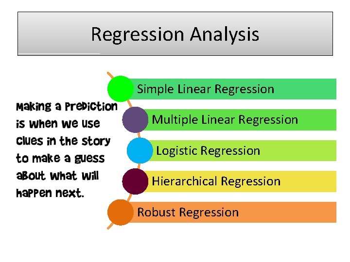
Regression Analysis Simple Linear Regression Multiple Linear Regression Logistic Regression Hierarchical Regression Robust Regression

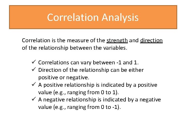
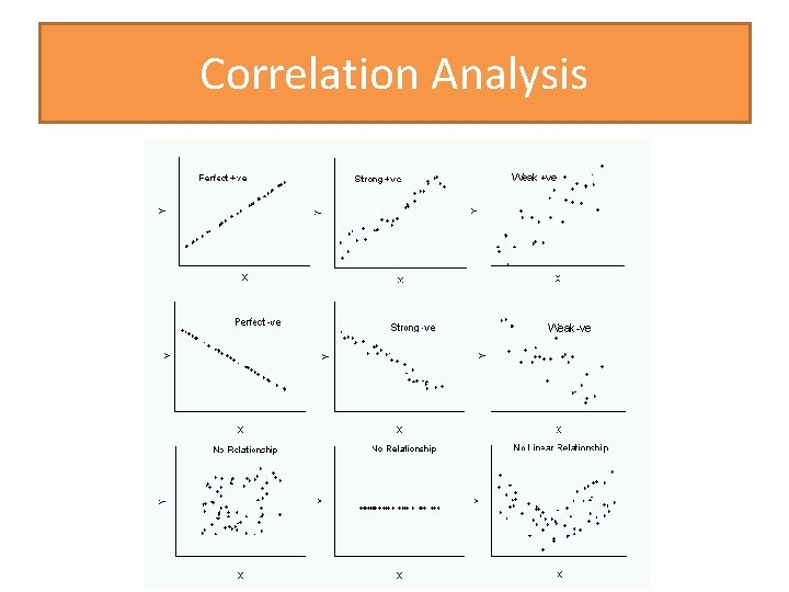
Correlation Analysis Correlation is the measure of the strength and direction of the relationship between the variables. ü Correlations can vary between -1 and 1. ü Direction of the relationship can be either positive or negative. ü A positive relationship is indicated by a positive value (e. g. , ranging from 0 to 1). ü A negative relationship is indicated by a negative value (e. g. , ranging from 0 to -1).

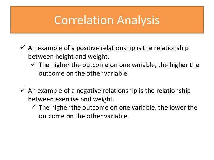
Correlation Analysis ü An example of a positive relationship is the relationship between height and weight. ü The higher the outcome on one variable, the higher the outcome on the other variable. ü An example of a negative relationship is the relationship between exercise and weight. ü The higher the outcome on one variable, the lower the outcome on the other variable.

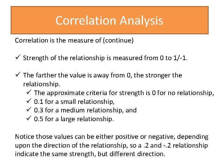
Correlation Analysis Correlation is the measure of (continue) ü Strength of the relationship is measured from 0 to 1/-1. ü The farther the value is away from 0, the stronger the relationship. ü The approximate criteria for strength is 0 for no relationship, ü 0. 1 for a small relationship, ü 0. 3 for a medium relationship, and ü 0. 5 for a large relationship. Notice those values can be either positive or negative, depending upon the direction of the relationship, so a. 2 and -. 2 relationship indicate the same strength, but different direction.

Correlation Analysis

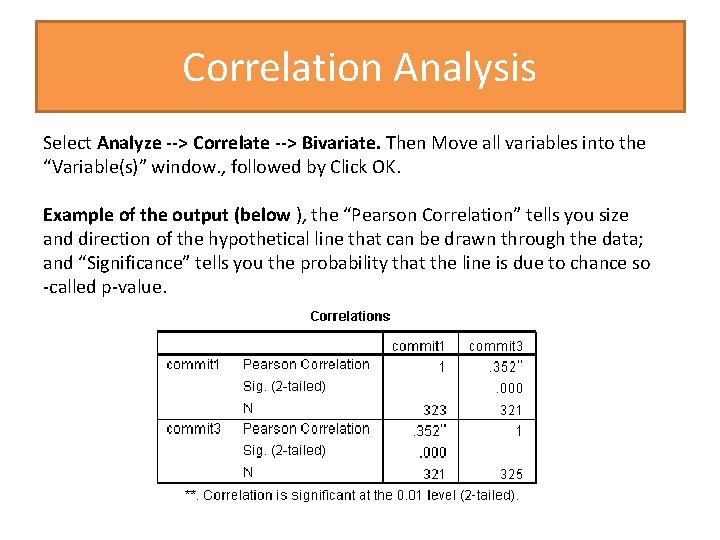
Correlation Analysis Select Analyze --> Correlate --> Bivariate. Then Move all variables into the “Variable(s)” window. , followed by Click OK. Example of the output (below ), the “Pearson Correlation” tells you size and direction of the hypothetical line that can be drawn through the data; and “Significance” tells you the probability that the line is due to chance so -called p-value.

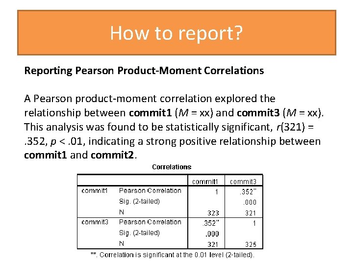
How to report? Reporting Pearson Product-Moment Correlations A Pearson product-moment correlation explored the relationship between commit 1 (M = xx) and commit 3 (M = xx). This analysis was found to be statistically significant, r(321) = . 352, p <. 01, indicating a strong positive relationship between commit 1 and commit 2.

Let’s try!

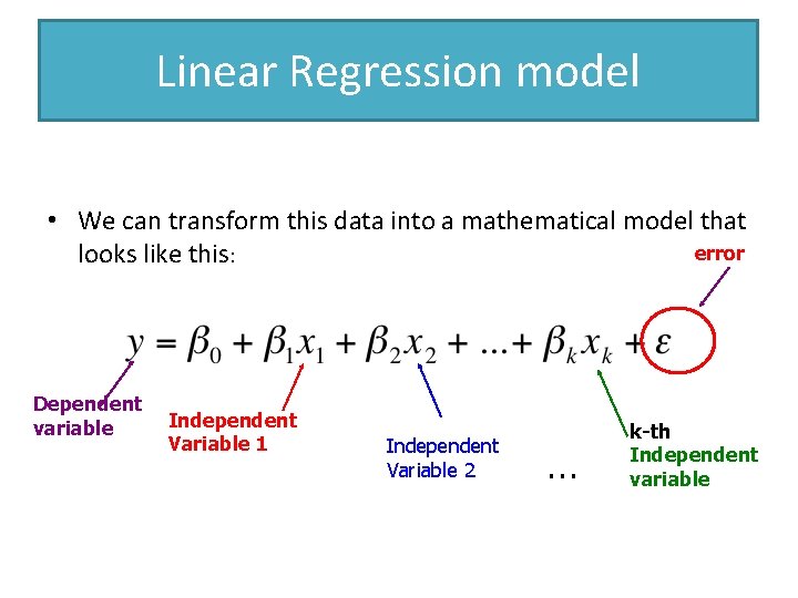
Linear Regression model • We can transform this data into a mathematical model that error looks like this: Dependent variable Independent Variable 1 Independent Variable 2 … k-th Independent variable

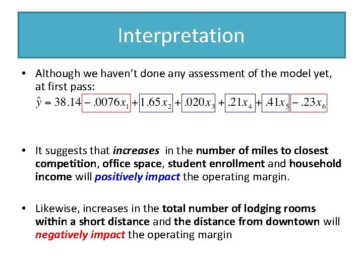
Interpretation • Although we haven’t done any assessment of the model yet, at first pass: • It suggests that increases in the number of miles to closest competition, office space, student enrollment and household income will positively impact the operating margin. • Likewise, increases in the total number of lodging rooms within a short distance and the distance from downtown will negatively impact the operating margin

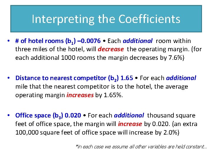
Interpreting the Coefficients • # of hotel rooms (b 1) – 0. 0076 • Each additional room within three miles of the hotel, will decrease the operating margin. (for each additional 1000 rooms the margin decreases by 7. 6%) • Distance to nearest competitor (b 2) 1. 65 • For each additional mile that the nearest competitor is to the hotel, the average operating margin increases by 1. 65%. • Office space (b 3) 0. 020 • For each additional thousand square feet of office space, the margin will increase by 0. 020. (an extra 100, 000 square feet of office space will increase by 2. 0%) *in each case we assume all other variables are held constant…

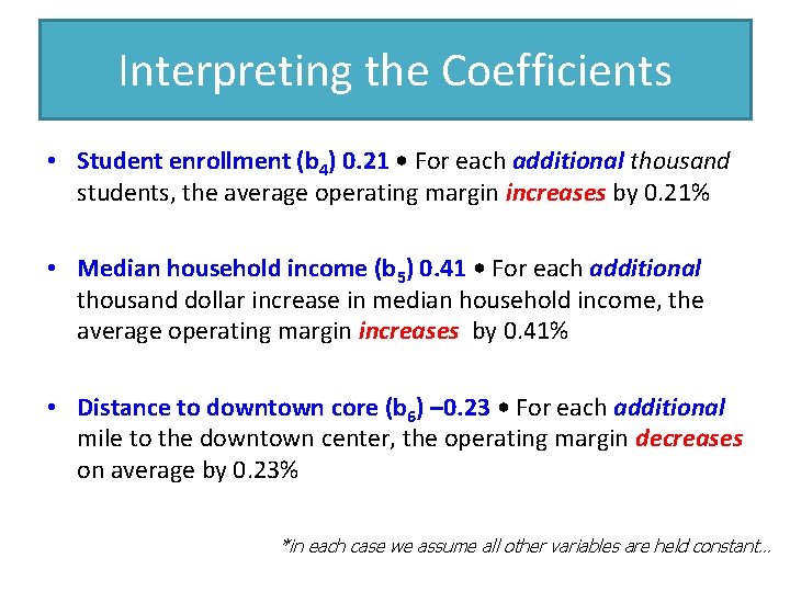
Interpreting the Coefficients • Student enrollment (b 4) 0. 21 • For each additional thousand students, the average operating margin increases by 0. 21% • Median household income (b 5) 0. 41 • For each additional thousand dollar increase in median household income, the average operating margin increases by 0. 41% • Distance to downtown core (b 6) – 0. 23 • For each additional mile to the downtown center, the operating margin decreases on average by 0. 23% *in each case we assume all other variables are held constant…

Let’s try

How good is your model?

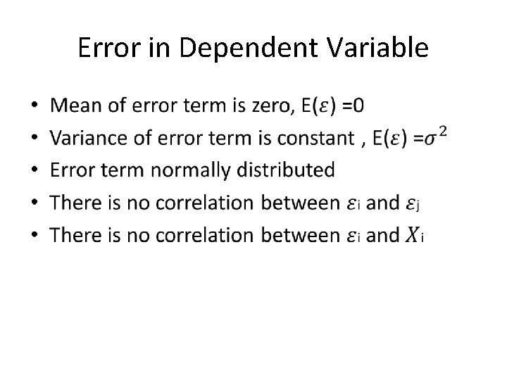
Error in Dependent Variable •

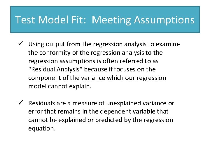
Test Model Fit: Meeting Assumptions ü Using output from the regression analysis to examine the conformity of the regression analysis to the regression assumptions is often referred to as "Residual Analysis" because if focuses on the component of the variance which our regression model cannot explain. ü Residuals are a measure of unexplained variance or error that remains in the dependent variable that cannot be explained or predicted by the regression equation.

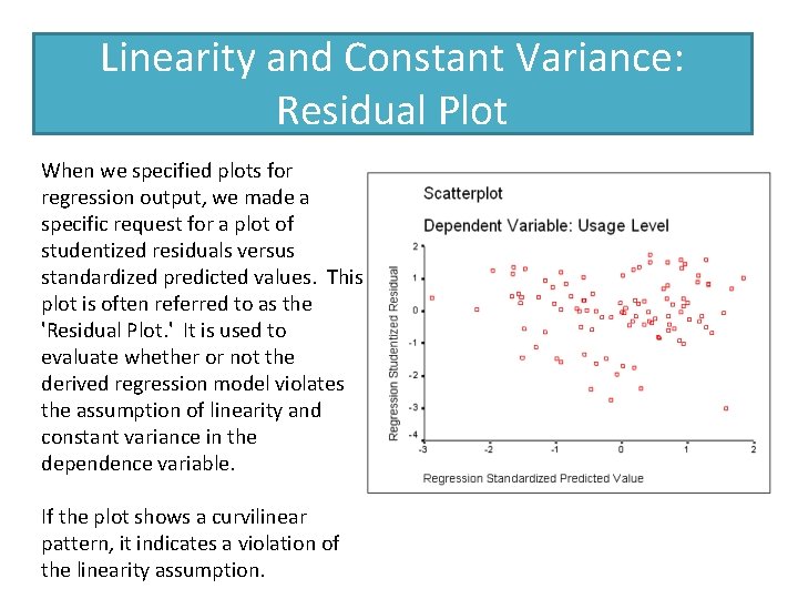
Linearity and Constant Variance: Residual Plot When we specified plots for regression output, we made a specific request for a plot of studentized residuals versus standardized predicted values. This plot is often referred to as the 'Residual Plot. ' It is used to evaluate whether or not the derived regression model violates the assumption of linearity and constant variance in the dependence variable. If the plot shows a curvilinear pattern, it indicates a violation of the linearity assumption.

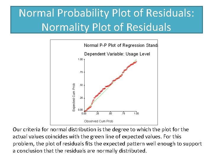
Normal Probability Plot of Residuals: Normality Plot of Residuals Our criteria for normal distribution is the degree to which the plot for the actual values coincides with the green line of expected values. For this problem, the plot of residuals fits the expected pattern well enough to support a conclusion that the residuals are normally distributed.

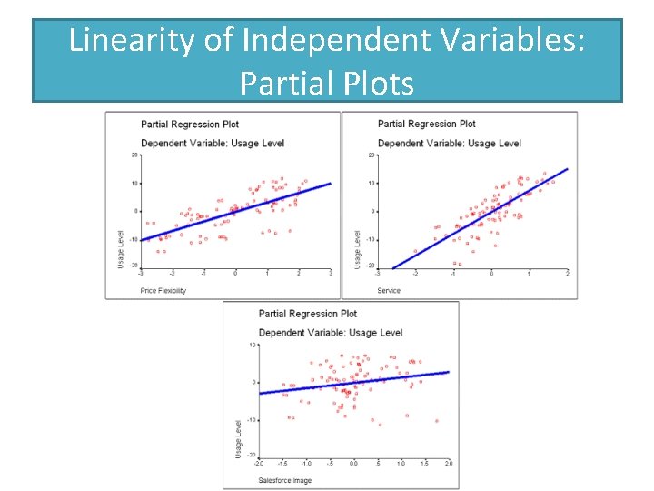
Linearity of Independent Variables: Partial Plots

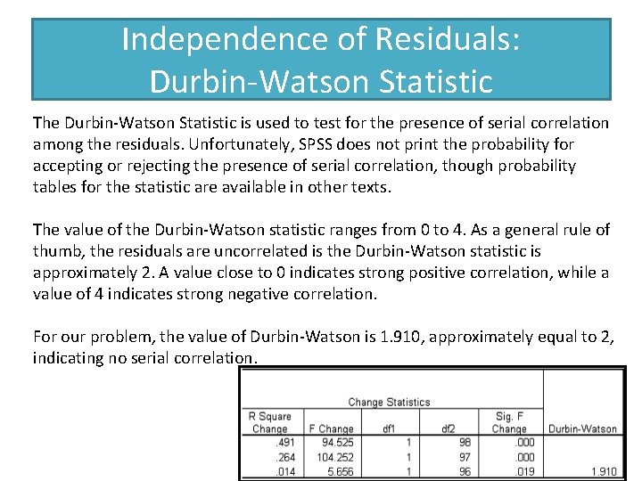
Independence of Residuals: Durbin-Watson Statistic The Durbin-Watson Statistic is used to test for the presence of serial correlation among the residuals. Unfortunately, SPSS does not print the probability for accepting or rejecting the presence of serial correlation, though probability tables for the statistic are available in other texts. The value of the Durbin-Watson statistic ranges from 0 to 4. As a general rule of thumb, the residuals are uncorrelated is the Durbin-Watson statistic is approximately 2. A value close to 0 indicates strong positive correlation, while a value of 4 indicates strong negative correlation. For our problem, the value of Durbin-Watson is 1. 910, approximately equal to 2, indicating no serial correlation.

Impact of Multicollinearity is a concern in our interpretation of the finding because it could lead us to mistakenly conclude that there was not a relationship between the dependent variable and one of the independent variables because a strong relationship between the independent variable and another independent variables in the analysis prevented the independent variable from demonstrating its relationship to the dependent variable. SPSS supports the detection of this problem by providing Tolerance statistics and the Variance Inflation Factor or VIF statistic, which is the inverse of tolerance. To detect problems of multicolllinearity, we look for tolerance values less than 0. 10 or VIF greater than 10 (1/0. 10=10). In a stepwise regression problem, SPSS will prevent a colinear variable from entering the solution by checking the tolerance of the variable at each step. To identify problems with multicollinearity, we check the tolerance or VIF for variables not included in the analysis after the last step.

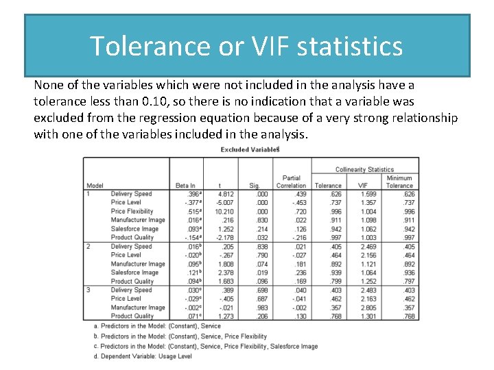
Tolerance or VIF statistics None of the variables which were not included in the analysis have a tolerance less than 0. 10, so there is no indication that a variable was excluded from the regression equation because of a very strong relationship with one of the variables included in the analysis.