Section VIII Simple Linear Regression Correlation Ex Riddle

Section VIII Simple Linear Regression & Correlation

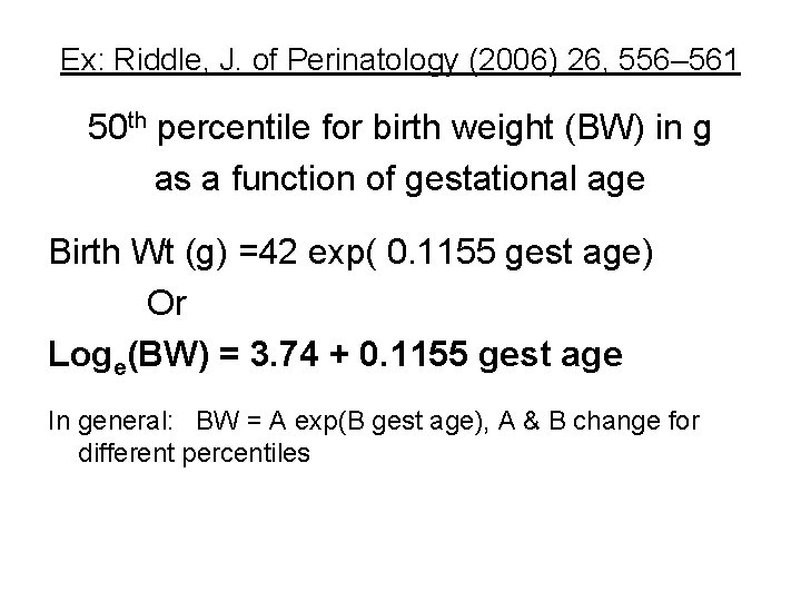
Ex: Riddle, J. of Perinatology (2006) 26, 556– 561 50 th percentile for birth weight (BW) in g as a function of gestational age Birth Wt (g) =42 exp( 0. 1155 gest age) Or Loge(BW) = 3. 74 + 0. 1155 gest age In general: BW = A exp(B gest age), A & B change for different percentiles

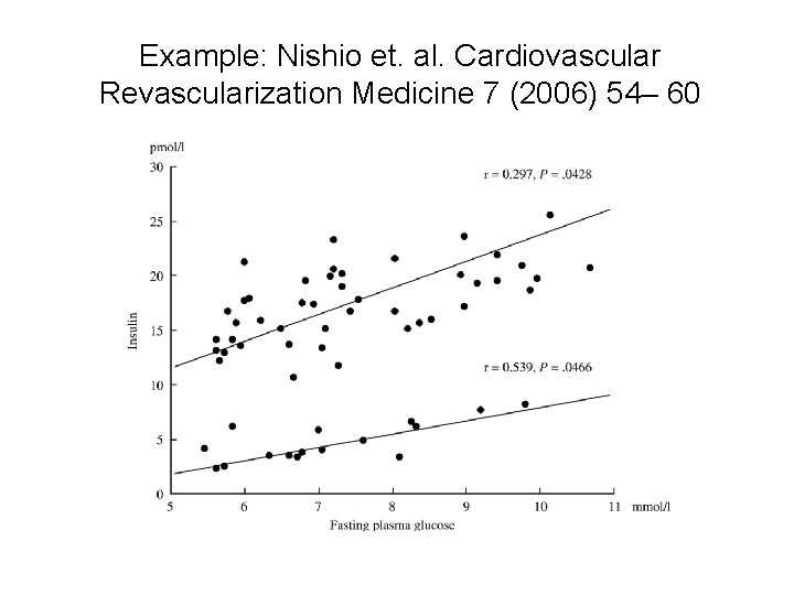
Example: Nishio et. al. Cardiovascular Revascularization Medicine 7 (2006) 54– 60

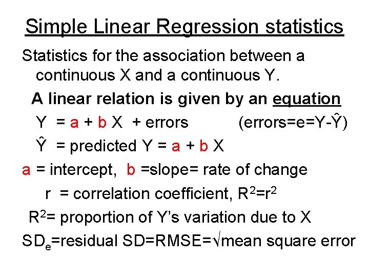
Simple Linear Regression statistics Statistics for the association between a continuous X and a continuous Y. A linear relation is given by an equation Y = a + b X + errors (errors=e=Y-Ŷ) Ŷ = predicted Y = a + b X a = intercept, b =slope= rate of change r = correlation coefficient, R 2=r 2 R 2= proportion of Y’s variation due to X SDe=residual SD=RMSE=√mean square error

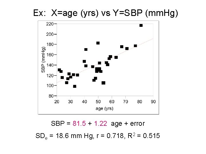
Ex: X=age (yrs) vs Y=SBP (mm. Hg) SBP = 81. 5 + 1. 22 age + error SDe = 18. 6 mm Hg, r = 0. 718, R 2 = 0. 515

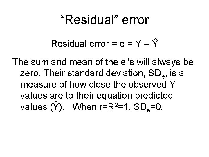
“Residual” error Residual error = e = Y – Ŷ The sum and mean of the ei’s will always be zero. Their standard deviation, SDe, is a measure of how close the observed Y values are to their equation predicted values (Ŷ). When r=R 2=1, SDe=0.

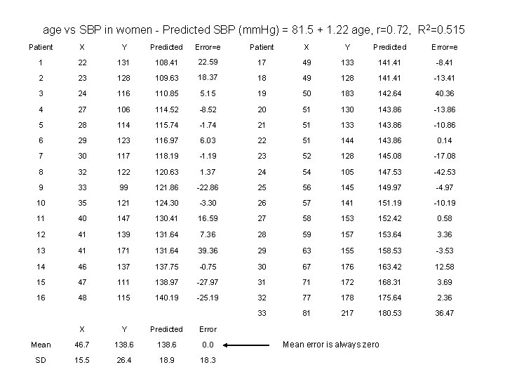
age vs SBP in women - Predicted SBP (mm. Hg) = 81. 5 + 1. 22 age, r=0. 72, R 2=0. 515 Patient X Y Predicted Error=e 1 22 131 108. 41 22. 59 17 49 133 141. 41 -8. 41 2 23 128 109. 63 18. 37 18 49 128 141. 41 -13. 41 3 24 116 110. 85 5. 15 19 50 183 142. 64 40. 36 4 27 106 114. 52 -8. 52 20 51 130 143. 86 -13. 86 5 28 114 115. 74 -1. 74 21 51 133 143. 86 -10. 86 6 29 123 116. 97 6. 03 22 51 144 143. 86 0. 14 7 30 117 118. 19 -1. 19 23 52 128 145. 08 -17. 08 8 32 120. 63 1. 37 24 54 105 147. 53 -42. 53 9 33 99 121. 86 -22. 86 25 56 145 149. 97 -4. 97 10 35 121 124. 30 -3. 30 26 57 141 151. 19 -10. 19 11 40 147 130. 41 16. 59 27 58 153 152. 42 0. 58 12 41 139 131. 64 7. 36 28 59 157 153. 64 3. 36 13 41 171 131. 64 39. 36 29 63 155 158. 53 -3. 53 14 46 137. 75 -0. 75 30 67 176 163. 42 12. 58 15 47 111 138. 97 -27. 97 31 71 172 168. 31 3. 69 16 48 115 140. 19 -25. 19 32 77 178 175. 64 2. 36 33 81 217 180. 53 36. 47 X Y Predicted Error Mean 46. 7 138. 6 0. 0 SD 15. 5 26. 4 18. 9 18. 3 Mean error is always zero

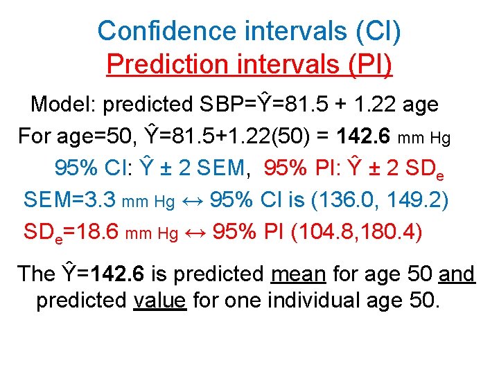
Confidence intervals (CI) Prediction intervals (PI) Model: predicted SBP=Ŷ=81. 5 + 1. 22 age For age=50, Ŷ=81. 5+1. 22(50) = 142. 6 mm Hg 95% CI: Ŷ ± 2 SEM, 95% PI: Ŷ ± 2 SDe SEM=3. 3 mm Hg ↔ 95% CI is (136. 0, 149. 2) SDe=18. 6 mm Hg ↔ 95% PI (104. 8, 180. 4) The Ŷ=142. 6 is predicted mean for age 50 and predicted value for one individual age 50.

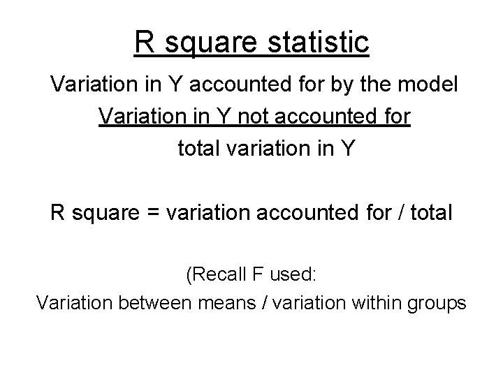
R square statistic Variation in Y accounted for by the model Variation in Y not accounted for total variation in Y R square = variation accounted for / total (Recall F used: Variation between means / variation within groups

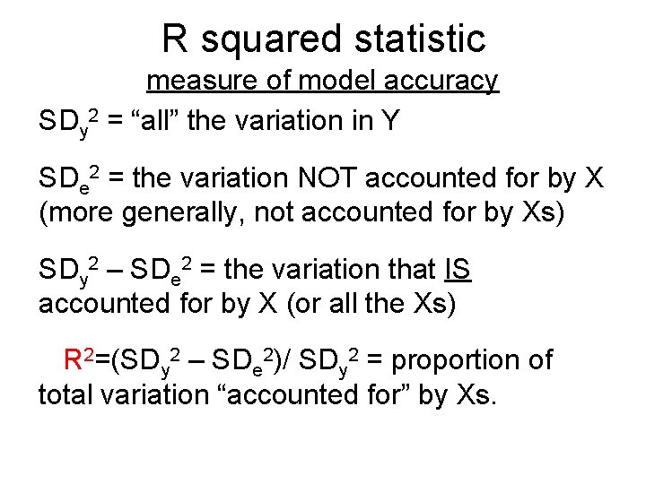
R squared statistic measure of model accuracy SDy 2 = “all” the variation in Y SDe 2 = the variation NOT accounted for by X (more generally, not accounted for by Xs) SDy 2 – SDe 2 = the variation that IS accounted for by X (or all the Xs) R 2=(SDy 2 – SDe 2)/ SDy 2 = proportion of total variation “accounted for” by Xs.

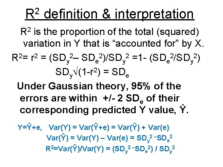
R 2 definition & interpretation R 2 is the proportion of the total (squared) variation in Y that is “accounted for” by X. R 2= r 2 = (SDy 2– SDe 2)/SDy 2 =1 - (SDe 2/SDy 2) SDy (1 -r 2) = SDe Under Gaussian theory, 95% of the errors are within +/- 2 SDe of their corresponding predicted Y value, Ŷ. Y=Ŷ+e, Var(Y) = Var(Ŷ+e) = Var(Ŷ) + Var(e) Var(Ŷ) = Var(Y) – Var(e) = SDy 2 –SDe 2 R 2=Var(Ŷ)/Var(Y) = (SDy 2 –SDe 2) / SDy 2

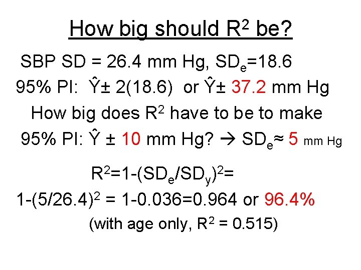
How big should 2 R be? SBP SD = 26. 4 mm Hg, SDe=18. 6 95% PI: Ŷ± 2(18. 6) or Ŷ± 37. 2 mm Hg How big does R 2 have to be to make 95% PI: Ŷ ± 10 mm Hg? SDe≈ 5 mm Hg R 2=1 -(SDe/SDy)2= 1 -(5/26. 4)2 = 1 -0. 036=0. 964 or 96. 4% (with age only, R 2 = 0. 515)

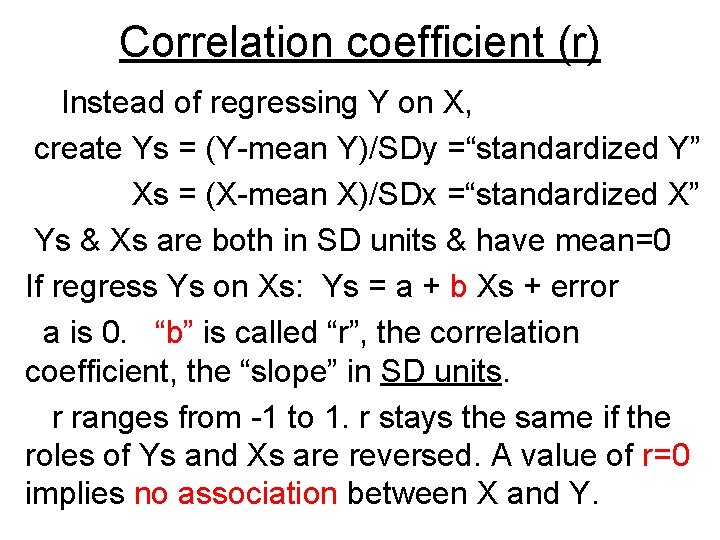
Correlation coefficient (r) Instead of regressing Y on X, create Ys = (Y-mean Y)/SDy =“standardized Y” Xs = (X-mean X)/SDx =“standardized X” Ys & Xs are both in SD units & have mean=0 If regress Ys on Xs: Ys = a + b Xs + error a is 0. “b” is called “r”, the correlation coefficient, the “slope” in SD units. r ranges from -1 to 1. r stays the same if the roles of Ys and Xs are reversed. A value of r=0 implies no association between X and Y.

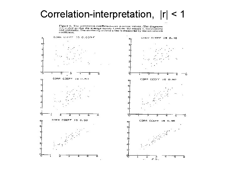
Correlation-interpretation, |r| < 1

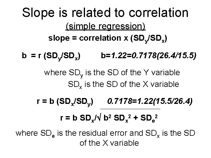
Slope is related to correlation (simple regression) slope = correlation x (SDy/SDx) b = r (SDy/SDx) b=1. 22=0. 7178(26. 4/15. 5) where SDy is the SD of the Y variable SDx is the SD of the X variable r = b (SDx/SDy) 0. 7178=1. 22(15. 5/26. 4) r = b SDx/ b 2 SDx 2 + SDe 2 where SDe is the residual error and SDx is the SD of the X variable

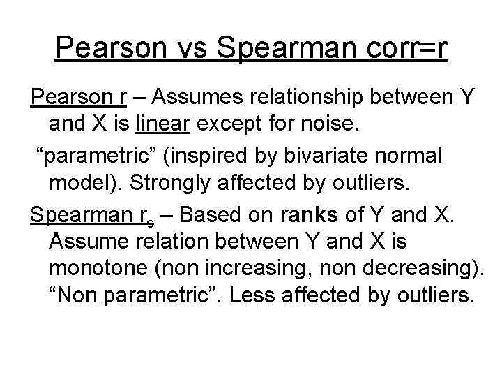
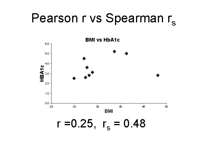
Pearson vs Spearman corr=r Pearson r – Assumes relationship between Y and X is linear except for noise. “parametric” (inspired by bivariate normal model). Strongly affected by outliers. Spearman rs – Based on ranks of Y and X. Assume relation between Y and X is monotone (non increasing, non decreasing). “Non parametric”. Less affected by outliers.

Pearson r vs Spearman rs BMI vs Hb. A 1 c 6. 0 HBA 1 c 5. 0 4. 0 3. 0 2. 0 1. 0 0. 0 25 30 35 40 45 BMI r =0. 25, rs = 0. 48 50

Limitation of linear models

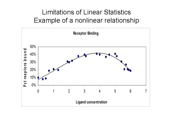
Limitations of Linear Statistics Example of a nonlinear relationship

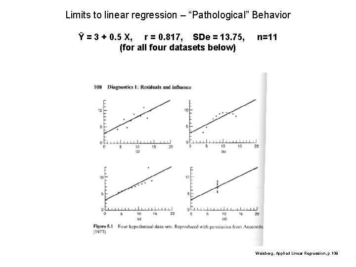
Limits to linear regression – “Pathological” Behavior Ŷ = 3 + 0. 5 X, r = 0. 817, SDe = 13. 75, (for all four datasets below) n=11 Weisberg, Applied Linear Regression, p 108

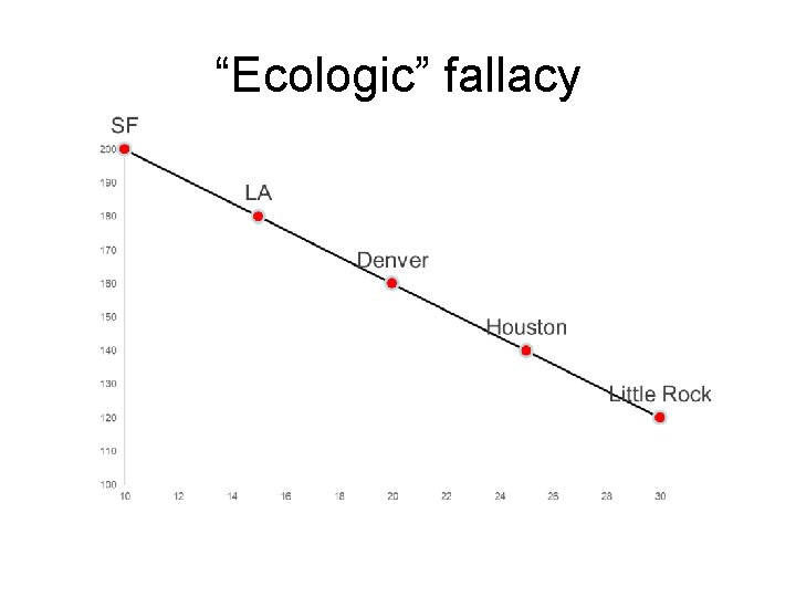
“Ecologic” fallacy

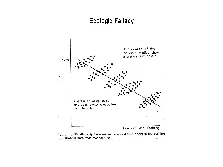
Ecologic Fallacy

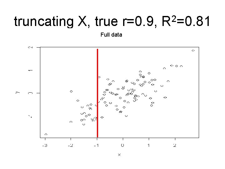
truncating X, true r=0. 9, R 2=0. 81 Full data

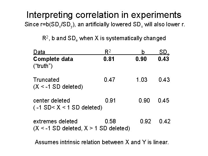
Interpreting correlation in experiments Since r=b(SDx/SDy), an artificially lowered SDx will also lower r. R 2, b and SDe when X is systematically changed Data Complete data (“truth”) R 2 0. 81 b 0. 90 SDe 0. 43 Truncated (X < -1 SD deleted) 0. 47 1. 03 0. 43 center deleted 0. 91 ( -1 SD< X < 1 SD deleted) 0. 90 0. 45 extremes deleted 0. 58 (X < -1 SD deleted, X > 1 SD deleted) 0. 92 0. 42 Assumes intrinsic relation between X and Y is linear.

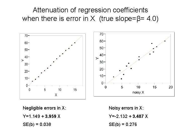
Attenuation of regression coefficients when there is error in X (true slope=β= 4. 0) Negligible errors in X: Noisy errors in X: Y=1. 149 + 3. 959 X Y=-2. 132 + 3. 487 X SE(b) = 0. 038 SE(b) = 0. 276

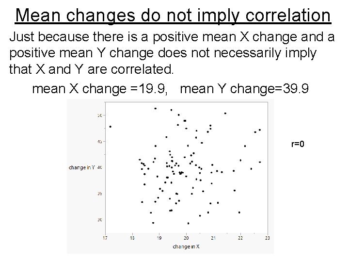
Mean changes do not imply correlation Just because there is a positive mean X change and a positive mean Y change does not necessarily imply that X and Y are correlated. mean X change =19. 9, mean Y change=39. 9 r=0

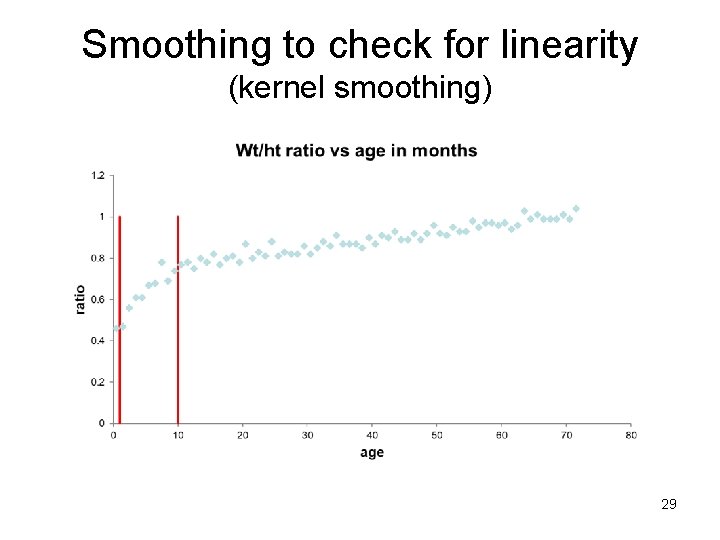
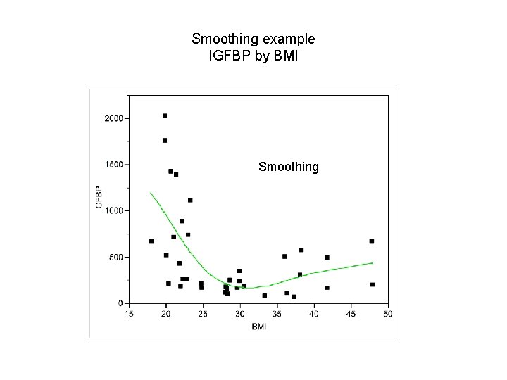
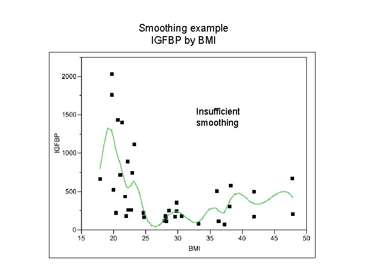
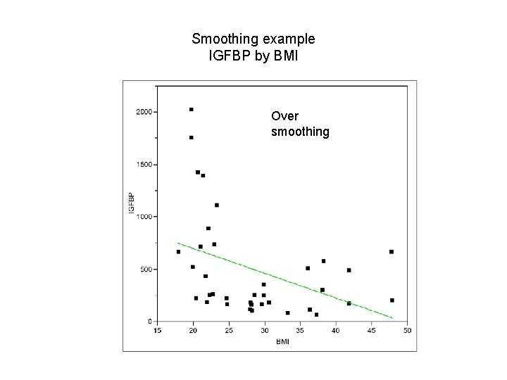
Checking for linearity – smoothing & splines Basic idea: In a plot of Y vs X, also plot Ŷ vs X where Ŷi = ∑ Wni Yi where ∑ Wni=1, Wni>0. The “weights” Wni, are larger near Yi and smaller far from Yi. Smooth: define a moving “window” of a given width around the ith data point and fit a mean (weighted moving average) in this window. Spline: break the X axis into non-overlapping bins and fit a polynomial within each bin such that the “ends” all “match”. The size of the window or bins control the amount of smoothing. We smooth until we obtain a smooth curve but go no further.

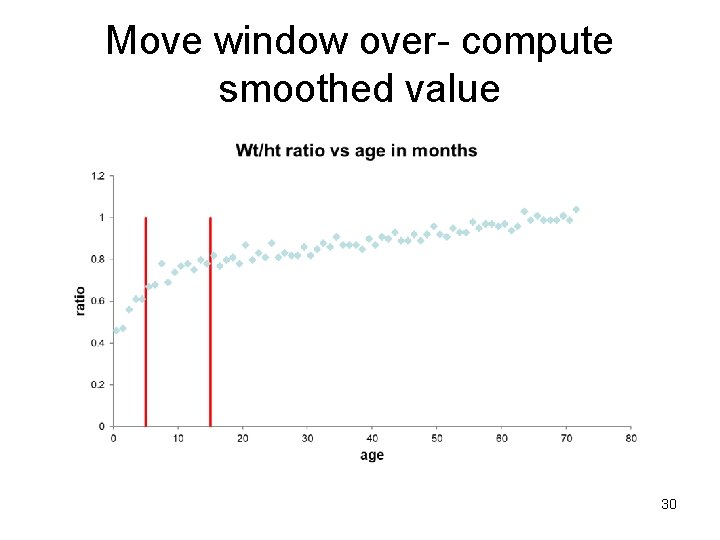
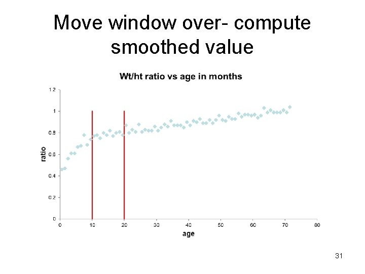
Check for linearity - Smoothing 1. Make a bin (window), take a (possibly weighted) average of all Y values in the bin or carry out a regression in the bin. The predicted value (mean) in the middle of the bin is the smoothed value (Ŷ). 2. Move bin over (overlapping) and repeat. 3. Connect the predicted values (Ŷs) with lines across all bins. 28

Smoothing to check for linearity (kernel smoothing) 29

Move window over- compute smoothed value 30

Move window over- compute smoothed value 31

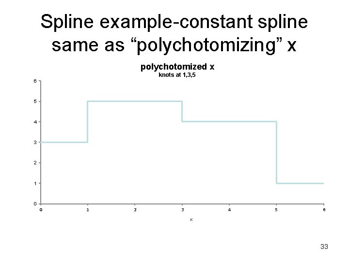
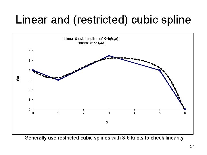
Splines to check for linearity Spline- Break the X axis into equally spaced non overlapping “bins” (segments). Fit a polynomial (usually a quadratic or cubic) within each bin such that Y at the “ends” (“knots”) all “match” (are piecewise continuous) and their first derivatives (slopes) are also continuous. 32

Spline example-constant spline same as “polychotomizing” x polychotomized x knots at 1, 3, 5 6 5 4 3 2 1 0 0 1 2 3 4 5 6 x 33

Linear and (restricted) cubic spline Linear & cubic spline of X=f(βs, x) "knots" at X=1, 3, 5 6 5 f(x) 4 3 2 1 0 0 1 2 3 4 5 6 X Generally use restricted cubic splines with 3 -5 knots to check linearity 34

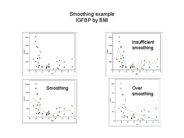
Smoothing example IGFBP by BMI Insufficient smoothing Smoothing Over smoothing

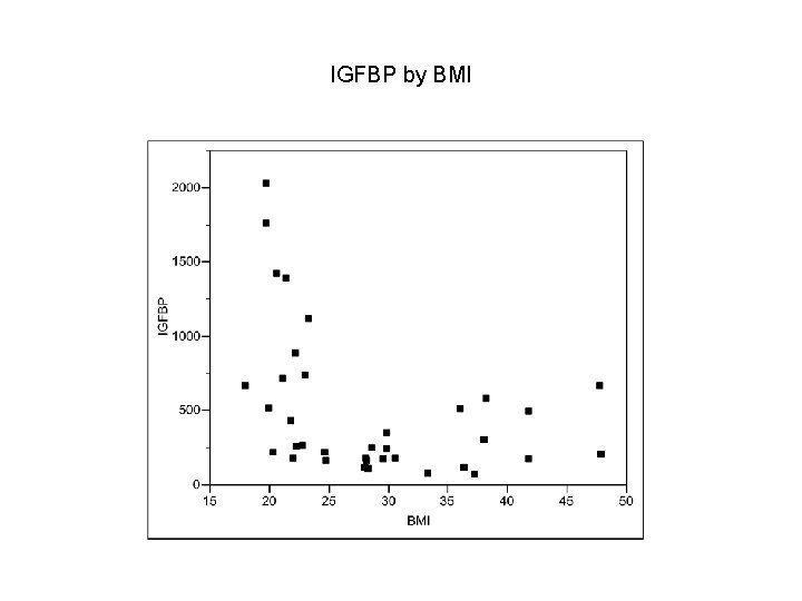
IGFBP by BMI

Smoothing example IGFBP by BMI Smoothing

Smoothing example IGFBP by BMI Insufficient smoothing

Smoothing example IGFBP by BMI Over smoothing

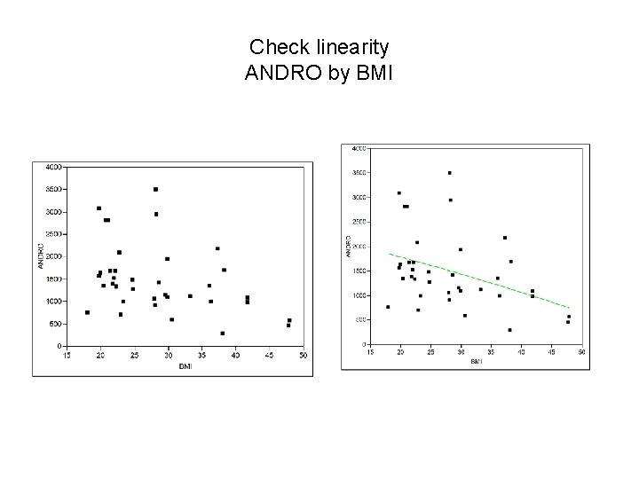
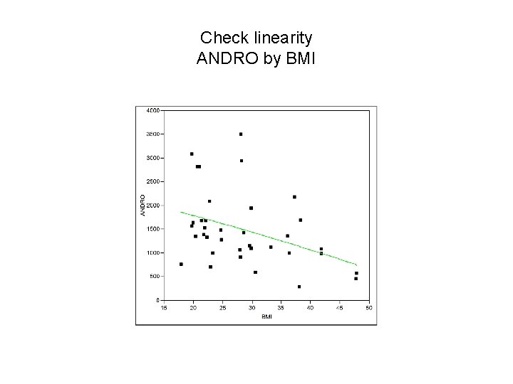
Check linearity ANDRO by BMI

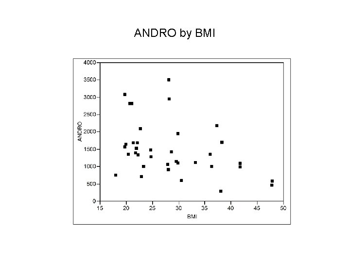
ANDRO by BMI

Check linearity ANDRO by BMI