10 601 Machine Learning Regression Outline Regression vs

10 -601 Machine Learning Regression

Outline • Regression vs Classification • Linear regression – another discriminative learning method – As optimization Gradient descent – As matrix inversion (Ordinary Least Squares) • Overfitting and bias-variance • Bias-variance decomposition for classification

What is regression?

Inputs Density Estimator Probability √ Inputs Classifier Predict category √ Inputs Where we are Regressor Predict real # Today

Regression examples

Prediction of menu prices Chaheau Gimpel … and Smith EMNLP 2012 …

A decision tree: classification Play Don’t Play

A regression tree Play ~= 37 Play ~= 5 Play ~= 0 Play = 30 m, 45 min Play = 0 m, 15 m Play = 0 m, 0 m Play ~= 32 Play = 20 m, 30 m, 45 m,

Theme for the week: learning as optimization

Types of learners • Two types of learners: 1. Generative: make assumptions about how to generate data (given the class) - e. g. , naïve Bayes 2. Discriminative - directly estimate a decision rule/boundary - e. g. , logistic regression Today: another discriminative learner, but for regression tasks

Least Mean Squares Regression for LMS as optimization Toy problem #2 11

Linear regression • Given an input x we would like to compute an output y • For example: - Predict height from age - Predict Google’s price from Yahoo’s price - Predict distance from wall from sensors Y X

Linear regression • Given an input x we would like to compute an output y • In linear regression we assume that y and x are related with the following equation: What we are trying to predict Y Observed values y = wx+ where w is a parameter and represents measurement or other noise X

Linear regression Y • Our goal is to estimate w from a training data of <xi, yi> pairs • Optimization goal: minimize squared error (least squares): X • Why least squares? - minimizes squared distance between measurements and predicted line - has a nice probabilistic interpretation - the math is pretty see HW

Solving linear regression • To optimize: • We just take the derivative w. r. t. to w …. prediction Compare to logistic regression…

Solving linear regression • To optimize – closed form: • We just take the derivative w. r. t. to w and set to 0: covar(X, Y)/var(X) if mean(X)=mean(Y)=0

Regression example • Generated: w=2 • Recovered: w=2. 03 • Noise: std=1

Regression example • Generated: w=2 • Recovered: w=2. 05 • Noise: std=2

Regression example • Generated: w=2 • Recovered: w=2. 08 • Noise: std=4

Bias term • So far we assumed that the line passes through the origin • What if the line does not? • No problem, simply change the model to y = w 0 + w 1 x+ Y w 0 • Can use least squares to determine w 0 , w 1 X

Multivariate regression • What if we have several inputs? - Stock prices for Yahoo, Microsoft and Ebay for the Google prediction task • This becomes a multivariate regression problem • Again, its easy to model: y = w 0 + w 1 x 1+ … + wkxk + Google’s stock price Microsoft’s stock price Yahoo’s stock price

Multivariate regression • What if we have several inputs? - Stock prices for Yahoo, Microsoft and Ebay for the Google prediction task • This becomes a multivariate regression problem • Again, its easy to model: y = w 0 + w 1 x 1+ … + wkxk +

Not all functions can be approximated by a line/hyperplane… y=10+3 x 12 -2 x 22+ In some cases we would like to use polynomial or other terms based on the input data, are these still linear regression problems? Yes. As long as the coefficients are linear the equation is still a linear regression problem!

Non-Linear basis function • So far we only used the observed values x 1, x 2, … • However, linear regression can be applied in the same way to functions of these values – Eg: to add a term w x 1 x 2 add a new variable z=x 1 x 2 so each example becomes: x 1, x 2, …. z • As long as these functions can be directly computed from the observed values the parameters are still linear in the data and the problem remains a multi-variate linear regression problem

Non-Linear basis function • How can we use this to add an intercept term? Add a new “variable” z=1 and weight w 0

Non-linear basis functions • What type of functions can we use? • A few common examples: - Polynomial: j(x) = xj for j=0 … n - Gaussian: - Sigmoid: - Logs: Any function of the input values can be used. The solution for the parameters of the regression remains the same.

General linear regression problem • Using our new notations for the basis function linear regression can be written as • Where j(x) can be either xj for multivariate regression or one of the non-linear basis functions we defined • … and 0(x)=1 for the intercept term

Learning/Optimizing Multivariate Least Squares Approach 1: Gradient Descent

Gradient descent 30

Gradient Descent for Linear Regression Goal: minimize the following loss function: sum over n examples sum over k+1 basis vectors

Gradient Descent for Linear Regression Goal: minimize the following loss function:

Gradient Descent for Linear Regression Learning algorithm: • Initialize weights w=0 • For t=1, … until convergence: • Predict for each example xi using w: • Compute gradient of loss: • This is a vector g • Update: w = w – λg • λ is the learning rate.

Gradient Descent for Linear Regression • We can use any of the tricks we used for logistic regression: – stochastic gradient descent (if the data is too big to put in memory) – regularization –…

Linear regression is a convex optimization problem so again gradient descent will reach a global optimum proof: differentiate again to get the second derivative

Multivariate Least Squares Approach 2: Matrix Inversion

OLS (Ordinary Least Squares Solution) Goal: minimize the following loss function:

Goal: minimize the following loss function: k+1 basis vectors Notation: n examples

Goal: minimize the following loss function: k+1 basis vectors n examples

k+1 basis vectors n examples …

k+1 basis vectors n examples …

k+1 basis vectors n examples …

n examples …

n examples k+1 basis …

k+1 basis vectors n examples …

recap: Solving linear regression • To optimize – closed form: • We just take the derivative w. r. t. to w and set to 0: covar(X, Y)/var(X) if mean(X)=mean(Y)=0

k+1 basis vectors n examples …

LMS for general linear regression problem Deriving w we get: n entries vector k+1 entries vector n by k+1 matrix This solution is also known as ‘pseudo inverse’ Another reason to start with an objective function: you can see when two learning methods are the same!

LMS versus gradient descent LMS solution: + Very simple in Matlab or something similar - Requires matrix inverse, which is expensive for a large matrix. Gradient descent: + Fast for large matrices + Stochastic GD is very memory efficient + Easily extended to other cases - Parameters to tweak (how to decide convergence? what is the learning rate? …. )

Regression and Overfitting

An example: polynomial basis vectors on a small dataset – From Bishop Ch 1

0 th Order Polynomial n=10

1 st Order Polynomial

3 rd Order Polynomial

9 th Order Polynomial

Over-fitting Root-Mean-Square (RMS) Error:

Polynomial Coefficients

Data Set Size: 9 th Order Polynomial

Regularization Penalize large coefficient values

Regularization: +

Polynomial Coefficients none exp(18) huge

Over Regularization:

Regularized Gradient Descent for LR Goal: minimize the following loss function:

Understanding Overfitting: Bias-Variance

Example Tom Dietterich, Oregon St

Example Tom Dietterich, Oregon St Same experiment, repeated: with 50 samples of 20 points each

noise is similar to error 1 The true function f can’t be fit perfectly with hypotheses from our class H (lines) Error 1 Fix: more expressive set of hypotheses H We don’t get the best hypothesis from H because of noise/small sample size Error 2 Fix: less expressive set of hypotheses H

Bias-Variance Decomposition: Regression

Bias and variance for regression • For regression, we can easily decompose the error of the learned model into two parts: bias (error 1) and variance (error 2) – Bias: the class of models can’t fit the data. • Fix: a more expressive model class. – Variance: the class of models could fit the data, but doesn’t because it’s hard to fit. • Fix: a less expressive model class.

Bias – Variance decomposition of error dataset and noise true function learned from D noise Fix test case x, then do this experiment: 1. Draw size n sample D=(x 1, y 1), …. (xn, yn) 2. Train linear regressor h. D using D 3. Draw one test example (x, f(x)+ε) 4. Measure squared error of h. D on that one example x What’s the expected error? 72

Bias – Variance decomposition of error Notation - to simplify this dataset and noise true function learned from D noise long-term expectation of learner’s prediction on this x averaged over many data sets D

Bias – Variance decomposition of error

Bias – Variance decomposition of error Squared difference between best possible prediction for x, f(x), and our “long-term” expectation for what the learner will do if we averaged over many datasets D, ED[h. D(x)] VARIANCE Squared difference btwn our longterm expectation for the learners performance, ED[h. D(x)], and what we expect in a representative run on a dataset D (hat y) BIAS 2 75

x=5 variance bias

Bias-variance decomposition • This is something real that you can (approximately) measure experimentally – if you have synthetic data • Different learners and model classes have different tradeoffs – large bias/small variance: few features, highly regularized, highly pruned decision trees, large-k k. NN… – small bias/high variance: many features, less regularization, unpruned trees, small-k k-NN…

Bias and variance • For classification, we can also decompose the error of a learned classifier into two terms: bias and variance – Bias: the class of models can’t fit the data. – Fix: a more expressive model class. – Variance: the class of models could fit the data, but doesn’t because it’s hard to fit. – Fix: a less expressive model class.

Another view of a decision tree Sepal_length<5. 7 Sepal_width>2. 8

Another view of a decision tree Sepal_length>5. 7 Sepal_width>2. 8 N length>4. 6 Y width>3. 1 length>5. 1 N Y

Background: “Bootstrap” sampling • Input: dataset D • Output: many variants of D: D 1, …, DT • For t=1, …. , T: – Dt = { } – For i=1…|D|: • Pick (x, y) uniformly at random from D (i. e. , with replacement) and add it to Dt • Some examples never get picked (~37%) • Some are picked 2 x, 3 x, ….

Measuring Bias-Variance with “Bootstrap” sampling • Create B bootstrap variants of D (approximate many draws of D) • For each bootstrap dataset – Tb is the dataset; Ub are the “out of bag” examples – Train a hypothesis hb on Tb – Test hb on each x in Ub • Now for each (x, y) example we have many predictions h 1(x), h 2(x), …. so we can estimate (ignoring noise) – variance: ordinary variance of h 1(x), …. , hn(x) – bias: average(h 1(x), …, hn(x)) - y

Bagging

Bootstrap Aggregation (Bagging) • Use the bootstrap to create B variants of D • Learn a classifier from each variant • Vote the learned classifiers to predict on a test example

Bagging (bootstrap aggregation) • Breaking it down: – input: dataset D and YFCL – output: a classifier h. D-BAG Note that you can use any learner you like! – use bootstrap to construct variants D 1, …, DT – for t=1, …, T: train YFCL on Dt to get ht You can also test ht on the “out of bag” examples – to classify x with h. D-BAG • classify x with h 1, …. , h. T and predict the most frequently predicted class for x (majority vote)

Experiments Freund and Schapire

solid: NB dashed: LR

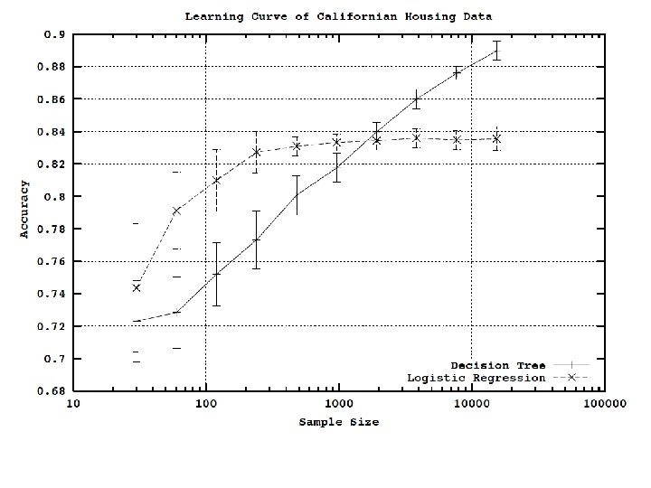
Bagged, minimally pruned decision trees

Generally, bagged decision trees outperform the linear classifier eventually if the data is large enough and clean enough.

Bagging (bootstrap aggregation) • �Experimentally: – especially with minimal pruning: decision trees have low bias but high variance. – bagging usually improves performance for decision trees and similar methods – It reduces variance without increasing the bias (much).