Topic 3 Simple Linear Regression Outline Simple linear

Topic 3: Simple Linear Regression

Outline • Simple linear regression model – Model parameters – Distribution of error terms • Estimation of regression parameters – Method of least squares – Maximum likelihood

Data for Simple Linear Regression • • Observe i=1, 2, . . . , n pairs of variables Each pair often called a case Yi = ith response variable Xi = ith explanatory variable

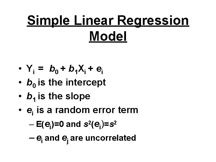
Simple Linear Regression Model • • Y i = b 0 + b 1 X i + e i b 0 is the intercept b 1 is the slope ei is a random error term – E(ei)=0 and s 2(ei)=s 2 – ei and ej are uncorrelated

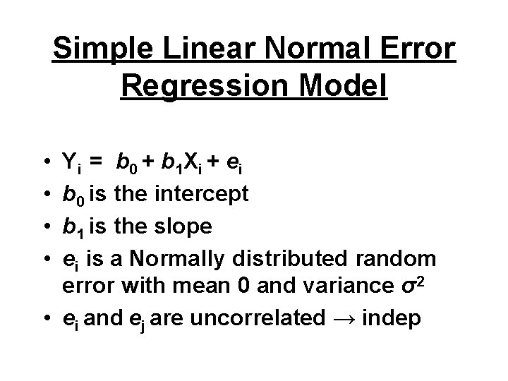
Simple Linear Normal Error Regression Model • • Y i = b 0 + b 1 X i + e i b 0 is the intercept b 1 is the slope ei is a Normally distributed random error with mean 0 and variance σ2 • ei and ej are uncorrelated → indep

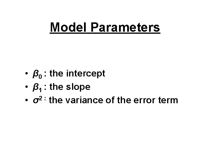
Model Parameters • β 0 : the intercept • β 1 : the slope • σ2 : the variance of the error term

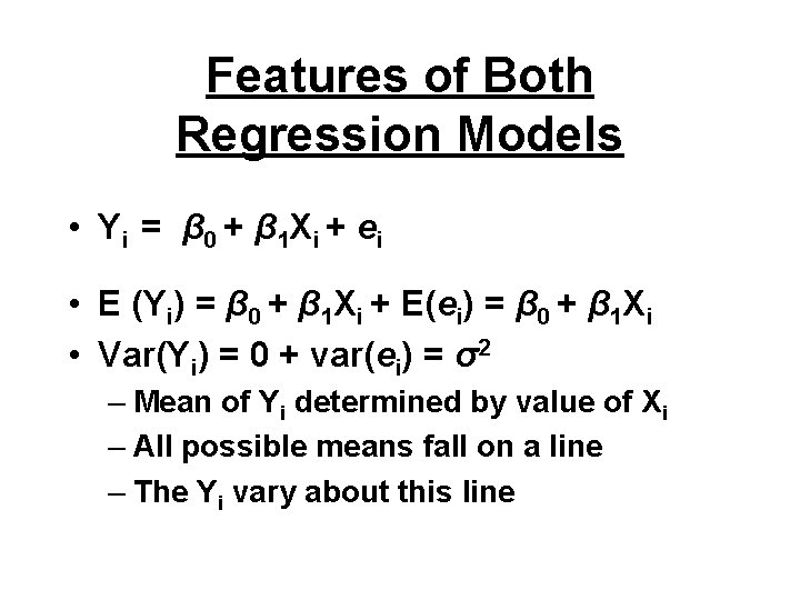
Features of Both Regression Models • Y i = β 0 + β 1 X i + e i • E (Yi) = β 0 + β 1 Xi + E(ei) = β 0 + β 1 Xi • Var(Yi) = 0 + var(ei) = σ2 – Mean of Yi determined by value of Xi – All possible means fall on a line – The Yi vary about this line

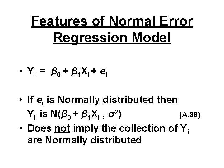
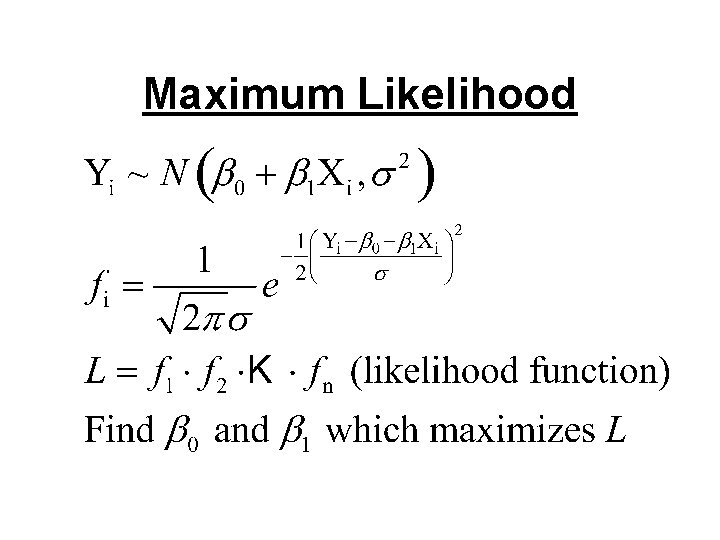
Features of Normal Error Regression Model • Y i = β 0 + β 1 X i + e i • If ei is Normally distributed then Yi is N(β 0 + β 1 Xi , σ2) (A. 36) • Does not imply the collection of Yi are Normally distributed

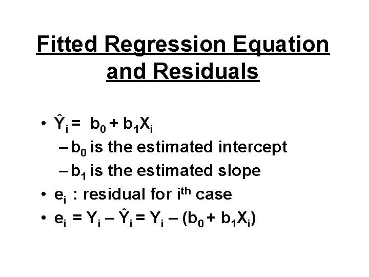
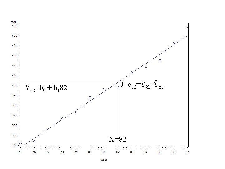
Fitted Regression Equation and Residuals • Ŷ i = b 0 + b 1 X i – b 0 is the estimated intercept – b 1 is the estimated slope • ei : residual for ith case • ei = Yi – Ŷi = Yi – (b 0 + b 1 Xi)

e 82=Y 82 -Ŷ 82=b 0 + b 182 X=82

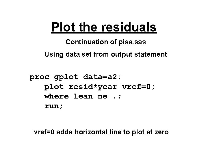
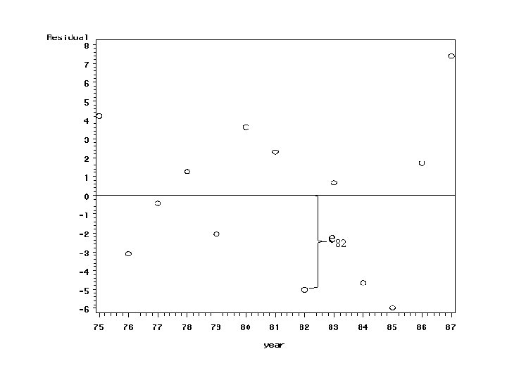
Plot the residuals Continuation of pisa. sas Using data set from output statement proc gplot data=a 2; plot resid*year vref=0; where lean ne. ; run; vref=0 adds horizontal line to plot at zero

e 82

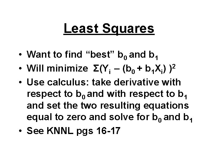
Least Squares • Want to find “best” b 0 and b 1 • Will minimize Σ(Yi – (b 0 + b 1 Xi) )2 • Use calculus: take derivative with respect to b 0 and with respect to b 1 and set the two resulting equations equal to zero and solve for b 0 and b 1 • See KNNL pgs 16 -17

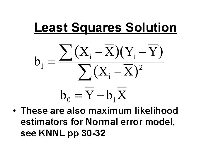
Least Squares Solution • These are also maximum likelihood estimators for Normal error model, see KNNL pp 30 -32

Maximum Likelihood

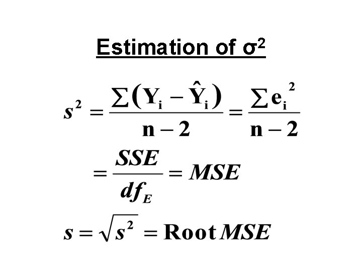
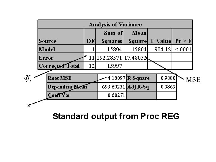
Estimation of σ2

Source Model Error Corrected Total dfe Analysis of Variance Sum of Mean DF Squares Square F Value Pr > F 1 15804 904. 12 <. 0001 11 192. 28571 17. 48052 12 15997 Root MSE Dependent Mean Coeff Var 4. 18097 R-Square 0. 9880 693. 69231 Adj R-Sq 0. 9869 0. 60271 s Standard output from Proc REG MSE

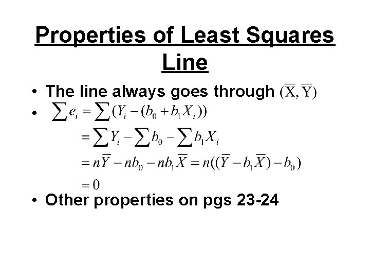
Properties of Least Squares Line • The line always goes through • • Other properties on pgs 23 -24

Background Reading • Chapter 1 – 1. 6 : Estimation of regression function – 1. 7 : Estimation of error variance – 1. 8 : Normal regression model • Chapter 2 – 2. 1 and 2. 2 : inference concerning ’s • Appendix A – A. 4, A. 5, A. 6, and A. 7