Econometrics Econ 405 Chapter 5 The Simple Regression

Econometrics Econ. 405 Chapter 5: The Simple Regression Model

I. Understanding the definition of Simple Linear Regression Model § There are two types of regression models (Simple vs. multiple regression models. § The simple regression model can be used to study the relationship between any two variables. § This simple regression model is appropriate as an empirical tool. § It is also a good practice for studying multiple regression model (covered next chapters).

§ The analysis of applied econometrics begins with following: Ø Y and X are two variables representing some population. Ø We are interested in “explaining Y in terms of x”. Ø Or similarly, studying “how much Y varies with changes in X”.

Recall: Explaining the variable y in terms of variable x Intercept Dependent variable, explained variable, response variable, predicted variable, and regressand Slope parameter Independent variable, explanatory variable, control variable, predictor variable, and regressor Error term, disturbance, and unobservables

Ø In order to estimate the regression model, data is needed: A random sample of observations The Simple Regression Model First observation Second observation Third observation Value of the explanatory variable of the i-th observation n-th observation Value of the dependent variable of the i-th observation

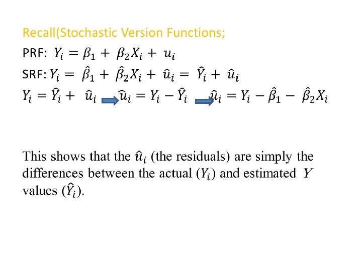
Ø Revist the regression equations:

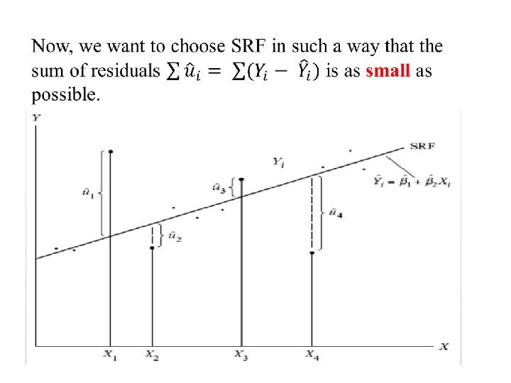
Ø Fit as good as possible a regression line through the data points: The Simple Regression Model Fitted regression line

II. Ordinary Least Squares Technique § Regression analysis refers to techniques that allow you to estimate economic relationship using data. § Mainly there are three techniques to estimate regression function; Generalized method of moments (GMM), Maximum Likelihood (ML), & Ordinary Least Squares (OLS). § The method used most frequently is commonly known as Ordinary Least Squares (OLS). § Although the OLS technique is popular and relatively simple, the application of it can become more complicated when starting to add more independent variables to your regression model.

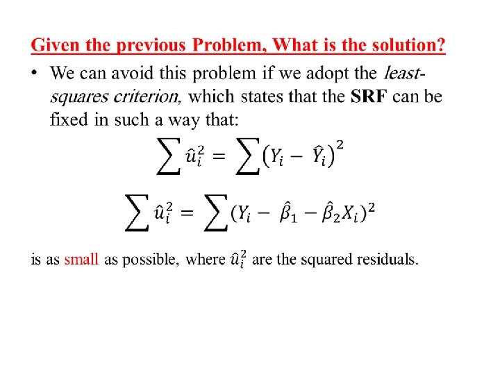
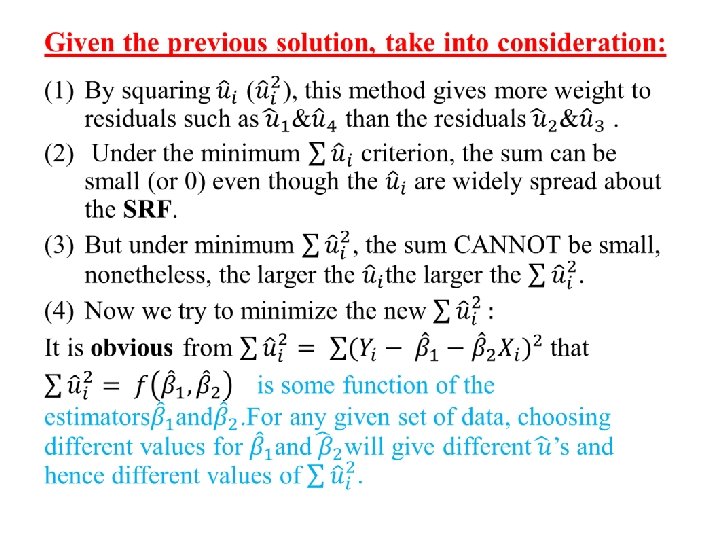
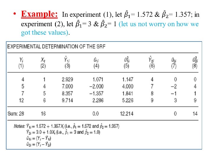
Ø Justifying the Least Squares Principle § When estimating a Sample Regression Function (SRF), the most common econometrics method to use is OLS. § Method of OLS uses the least squares principle to fit pre-specified regression. § The least squares principle states that SRF should be constructed ( with constant and slope function) so that the sum of squared distance between the observed values of “Y” and the values estimated from your SRF is minimized (the smallest possible value).

Ø Reasons for OLS Popularity A) OLS is easier than alternatives: Although other alternative methods are used to estimate same regression functions, they require more mathematical sophistication.

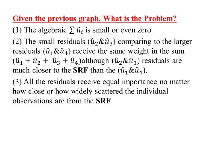
B) The OLS is sensible: So by using square residuals, you can avoid positive and negative residuals canceling each other out and find a regression line that’s as close as possible to the observed data points. How? ?

Ø The numerical properties of estimators obtained by the method of OLS: • The OLS estimators are expressed only in terms of the observable quantities (i. e. , X and Y). Therefore, they can be easily computed. • They are point estimators; that is, given the sample, each estimator will provide only a single (point, not interval) value of the relevant population parameter. • Once the OLS estimates are obtained from the sample data, the sample regression line can be easily obtained.

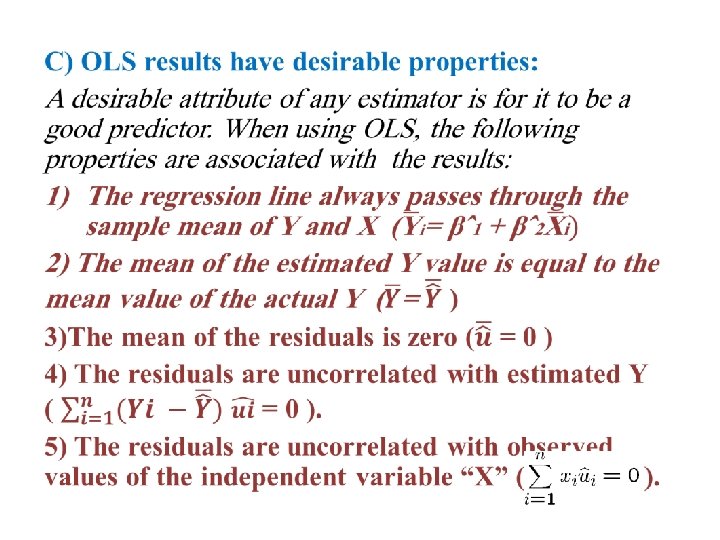
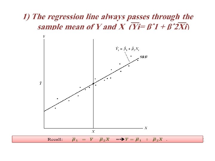
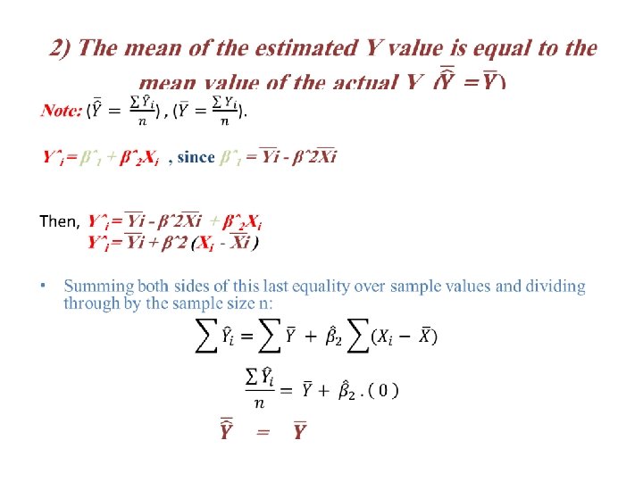
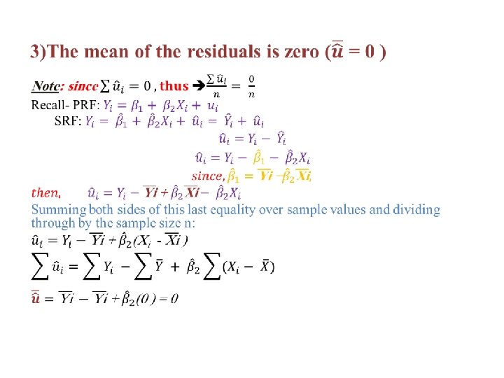
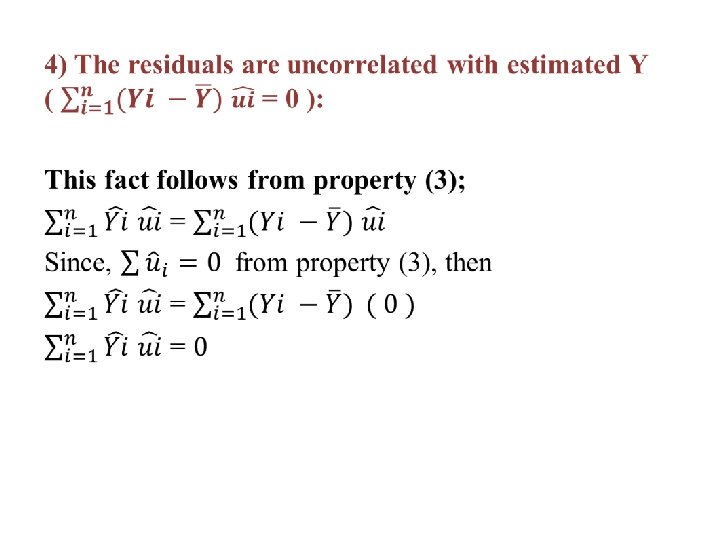
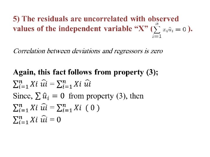
Recall: • Algebraic properties of OLS regression Fitted or predicted values Deviations from regression line sum up to zero Deviations from regression line (= residuals) Correlation between deviations and regressors is zero Sample averages of y and x lie on regression line

Accordingly: q Thus the Goodness-of-Fit is measures of variation to to show “How well does the explanatory variable explain the dependent variable? “ § TSS= total sum of squares § ESS= explained sum of squares § RSS= residual sum of squares

Total sum of squares, represents total variation in dependent variable Explained sum of squares, represents variation explained by regression Residual sum of squares, represents variation not explained by regression

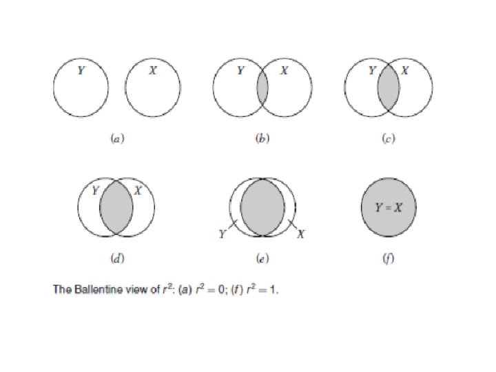
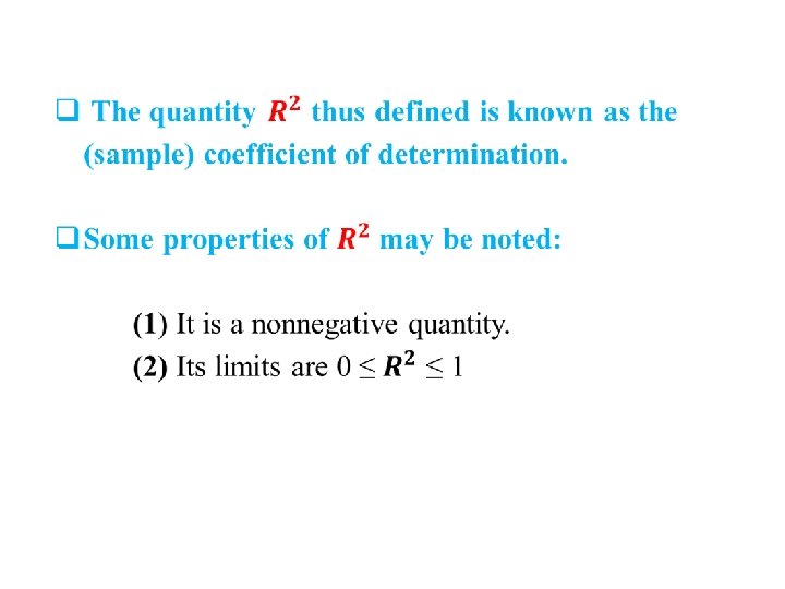
• Total variation Explained part R-squared measures the fraction of the total variation that is explained by the regression Unexplained part

III. OLS Assumptions- Classical Linear Regression Model (CLRM) § In regression analysis our objective is not only to obtain βˆ1 and βˆ2 but also to draw inferences about the true β 1 and β 2. For example, we would like to know how close βˆ1 and βˆ2 are to their counterparts in the population or how close Yˆi is to the true E(Y | Xi). § The econometrics model shows that Yi depends on both Xi and ui. The assumptions made about the Xi variable(s) and the error term are extremely critical to the valid interpretation of the regression estimates. § When deciding whether OLS is the best technique for your estimation problem, some requirements must be met. § They are called the OLS assumptions or the classical linear regression model (CLRM).

ØFirst Assumption: Keep in mind that the regressand Y and the regressor X themselves may be nonlinear.

ØSecond Assumption: This means the regression analysis is conditional on the given values of the regressor(s) X.

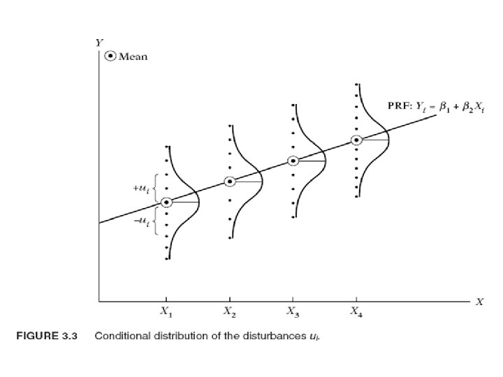
ØThird Assumption: • Revisit property (3); each Y population corresponding to a given X is distributed around its mean value with some Y values above the mean and some below it. the mean value of these deviations corresponding to any given X should be zero. Note that the assumption E(ui | Xi) = 0 implies that E(Yi | Xi) = β 1 + β 2 Xi.

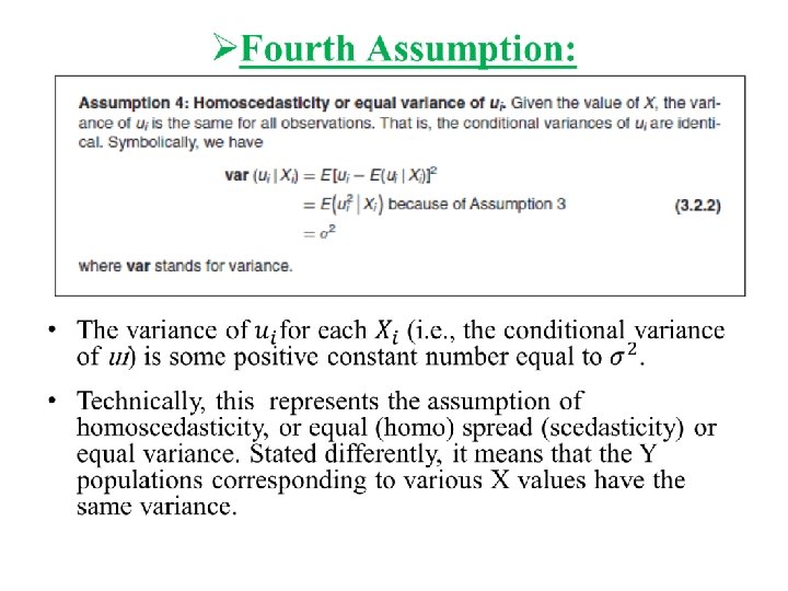
This situation, the variation around the regression line (which is the line of average relationship between Y and X) is the same across the X values; it neither increases or decreases as X varies.

The conditional variance of the Y population varies with X. This situation is known as heteroscedasticity, or unequal spread, or variance. Symbolically, in this situation Assumption (4) can be written as var (ui | Xi) = σ2 i var (u| X 1) < var (u| X 2), . . . , < var (u| Xi). Therefore, the likelihood is that the Y observations coming from the population with X = X 1 would be closer to the PRF than those coming from populations corresponding to X = X 2, X = X 3, and so on. In short, not all Y values corresponding to the various X’s will be equally reliable, reliability being judged by how closely or distantly the Y values are distributed around their means, that is, the points on the PRF.

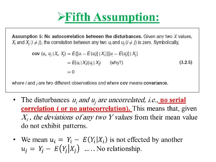
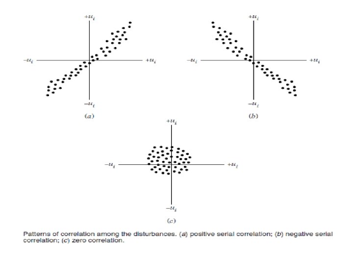
According to the Figures , When the disturbances (deviations) follow systematic patterns: q. In Figure a, we see that the u’s are positively correlated, a positive u followed by a positive u or a negative u followed by a negative u. q. In Figure b, the u’s are negatively correlated, a positive u followed by a negative u and vice versa. We can see there is auto- or serial correlation. q. In Figure c, shows that there is no systematic pattern to the u’s, thus indicating zero correlation. In another word, auto- or serial correlation, is absent.

ØSixth Assumption: § The disturbance u and explanatory variable X are uncorrelated. The it is assumed that X and u (which may represent the influence of all the omitted variables) have separate (and additive) influence on Y. § But if X and u are correlated, it is not possible to assess their individual effects on Y. Thus, if X and u are positively correlated, X increases when u increases and it decreases when u decreases. Similarly, if X and u are negatively correlated, X increases when u decreases and it decreases when u increases. In either case, it is difficult to isolate the influence of X and u on Y

ØSeventh Assumption: • Note: n > # of X's , n > # of β's

Ø Eight Assumption: •

ØNinth Assumption: (1) What variables should be included in the model? (2) What is the functional form of the model? Is it linear in the parameters, the variables, or both? (3) What are the probabilistic assumptions made about the Yi , the Xi, and the ui entering the model?

ØTenth Assumption: § For models beyond the two-variable model containing several regressors (discussed next chapter).

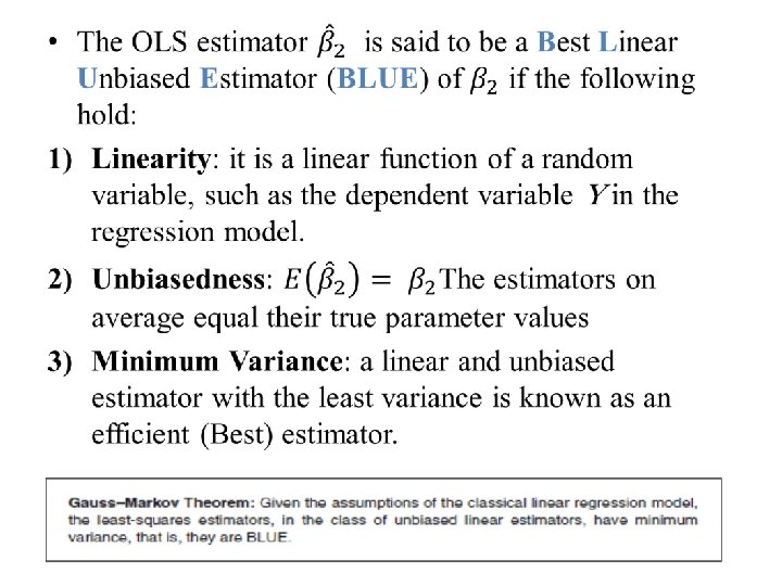
IV. Gauss–Markov Theorem •

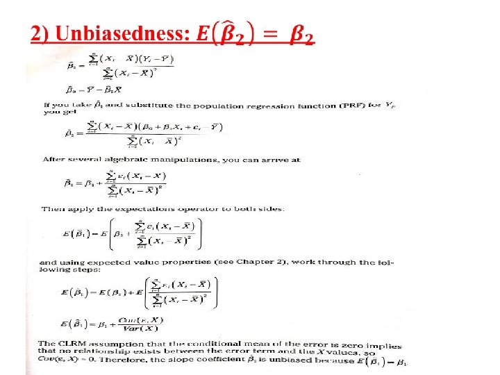
Similarly it can be shown that for β 1 too.

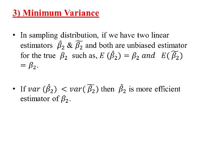
• According to the graphs: • For convenience, assume that β*2, like βˆ2, is unbiased, that is, its average or expected value is equal to β 2. Assume further that both βˆ2 and β*2 are linear estimators, that is, they are linear functions of Y. Which estimator, βˆ2 or β*2, would you choose? • To answer this question, It is obvious that although both βˆ2 and β*2 are unbiased the distribution of β*2 is more diffused or widespread around the mean value than the distribution of βˆ2. In other words, the variance of β*2 is larger than the variance of βˆ2. • Now given two estimators that are both linear and unbiased, one would choose the estimator with the smaller variance because it is more likely to be close to β 2 than the alternative estimator. In short, one would choose the BLUE estimator.

IIV. Evaluating Fit versus Quality • In economic settings, a high R² (close to 1 may indicate a violation in assumptions) is more likely to indicate something wrong with the regression instead of showing a high quality results. • Why not using R² as the only measure of your regression’s quality: – You may have high R² BUT no meaningful interpretation ( Check the validity of your economic theory). – Using small dataset ( or incorrect data) can lead to high R² value but deceptive results.