Econometrics Econ 405 Chapter 4 The Nature of

Econometrics Econ. 405 Chapter 4: The Nature of Regression Analysis

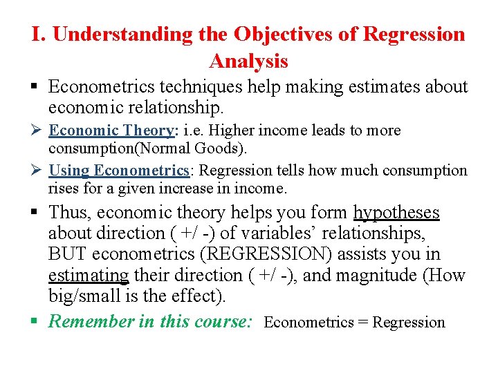
I. Understanding the Objectives of Regression Analysis § Econometrics techniques help making estimates about economic relationship. Ø Economic Theory: i. e. Higher income leads to more consumption(Normal Goods). Ø Using Econometrics: Regression tells how much consumption rises for a given increase in income. § Thus, economic theory helps you form hypotheses about direction ( +/ -) of variables’ relationships, BUT econometrics (REGRESSION) assists you in estimating their direction ( +/ -), and magnitude (How big/small is the effect). § Remember in this course: Econometrics = Regression

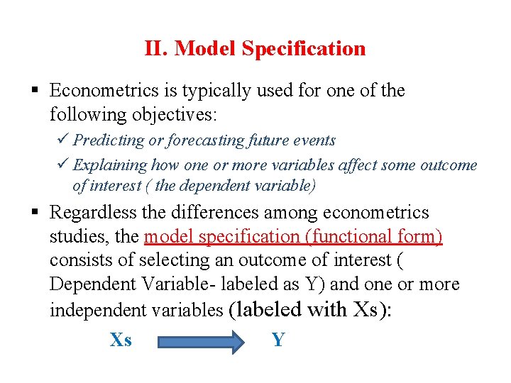
II. Model Specification § Econometrics is typically used for one of the following objectives: ü Predicting or forecasting future events ü Explaining how one or more variables affect some outcome of interest ( the dependent variable) § Regardless the differences among econometrics studies, the model specification (functional form) consists of selecting an outcome of interest ( Dependent Variable- labeled as Y) and one or more independent variables (labeled with Xs): Xs Y

§ The econometrics model should be justified: ØBe able to explain why it makes sense to think your dependent variable is caused by the independent variables you have selected. ØYou need to invest time explaining how independent variables are related to the outcome. ØRemember: regression analysis identifies the direction (+/-) and magnitude (big/small)of the relationship

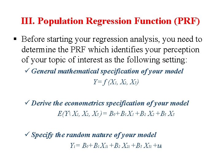
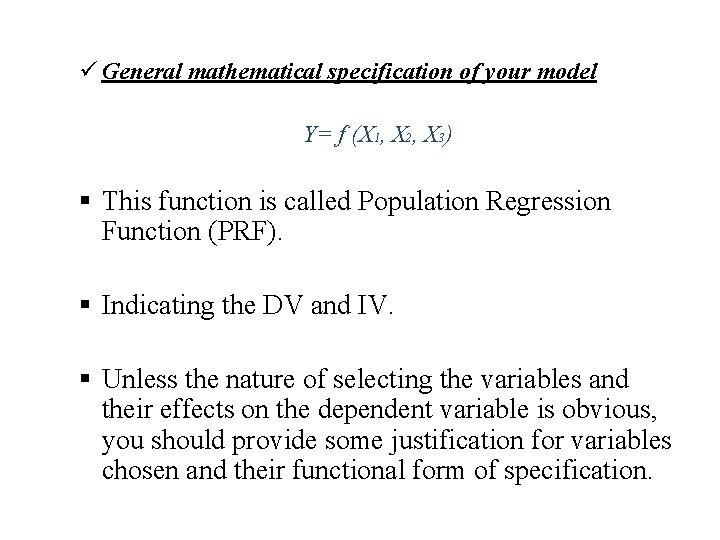
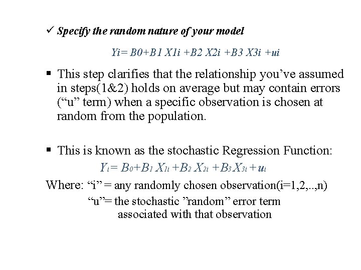
III. Population Regression Function (PRF) § Before starting your regression analysis, you need to determine the PRF which identifies your perception of your topic of interest as the following setting: ü General mathematical specification of your model Y= f (X 1, X 2, X 3) ü Derive the econometrics specification of your model E(Y X 1, X 2, X 3 )= B 0+B 1 X 1 +B 2 X 2 +B 3 X 3 ü Specify the random nature of your model Yi= B 0+B 1 X 1 i +B 2 X 2 i +B 3 X 3 i +ui

ü General mathematical specification of your model Y= f (X 1, X 2, X 3) § This function is called Population Regression Function (PRF). § Indicating the DV and IV. § Unless the nature of selecting the variables and their effects on the dependent variable is obvious, you should provide some justification for variables chosen and their functional form of specification.

ü Derive the econometrics specification of your model E(Y X 1, X 2, X 3 )= B 0+B 1 X 1 +B 2 X 2 +B 3 X 3 § Assuming linear model § The conditional mean E(Y X 1, X 2, X 3 ) indicates that the relationship is expected to hold, on average, for given values of the independent variables.

ü Specify the random nature of your model Yi= B 0+B 1 X 1 i +B 2 X 2 i +B 3 X 3 i +ui § This step clarifies that the relationship you’ve assumed in steps(1&2) holds on average but may contain errors (“u” term) when a specific observation is chosen at random from the population. § This is known as the stochastic Regression Function: Yi= B 0+B 1 X 1 i +B 2 X 2 i +B 3 X 3 i +ui Where: “i” = any randomly chosen observation(i=1, 2, . . , n) “u”= the stochastic ”random” error term associated with that observation

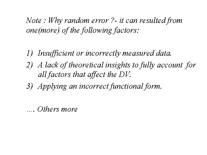
Note : Why random error ? - it can resulted from one(more) of the following factors: 1) Insufficient or incorrectly measured data. 2) A lack of theoretical insights to fully account for all factors that affect the DV. 3) Applying an incorrect functional form. …. Others more

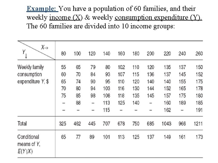
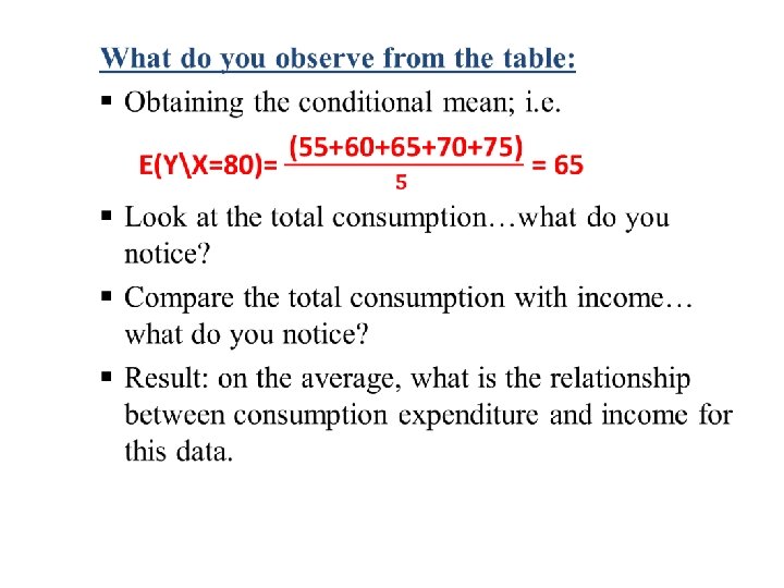
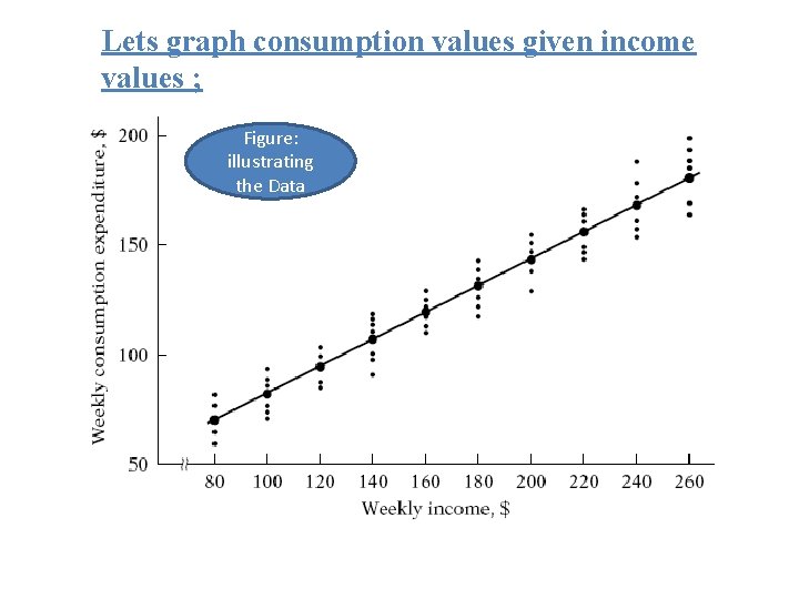
Example: You have a population of 60 families, and their weekly income (X) & weekly consumption expenditure (Y). The 60 families are divided into 10 income groups:

Lets graph consumption values given income values ; Figure: illustrating the Data

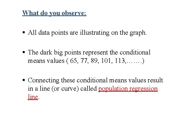
What do you observe: § All data points are illustrating on the graph. § The dark big points represent the conditional means values ( 65, 77, 89, 101, 113, ……. ) § Connecting these conditional means values result in a line (or curve) called population regression line.

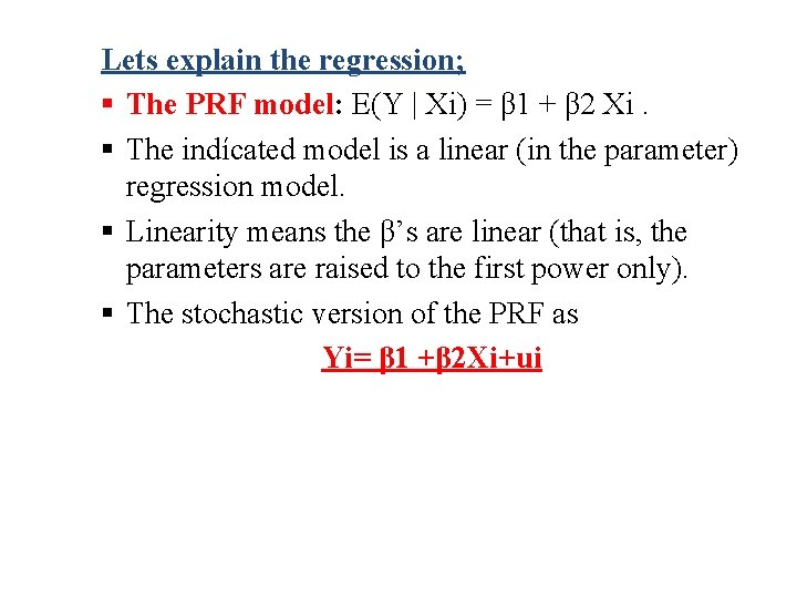
Lets explain the regression; § The PRF model: E(Y | Xi) = β 1 + β 2 Xi. § The indícated model is a linear (in the parameter) regression model. § Linearity means the β’s are linear (that is, the parameters are raised to the first power only). § The stochastic version of the PRF as Yi= β 1 +β 2 Xi+ui

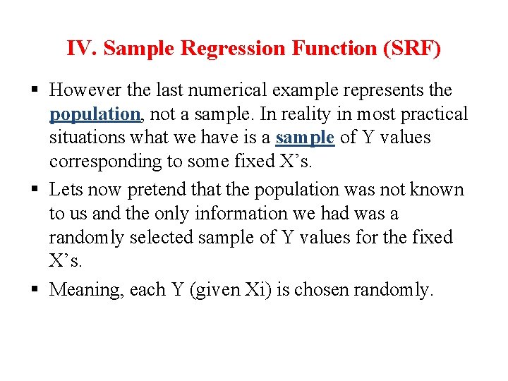
IV. Sample Regression Function (SRF) § However the last numerical example represents the population, not a sample. In reality in most practical situations what we have is a sample of Y values corresponding to some fixed X’s. § Lets now pretend that the population was not known to us and the only information we had was a randomly selected sample of Y values for the fixed X’s. § Meaning, each Y (given Xi) is chosen randomly.

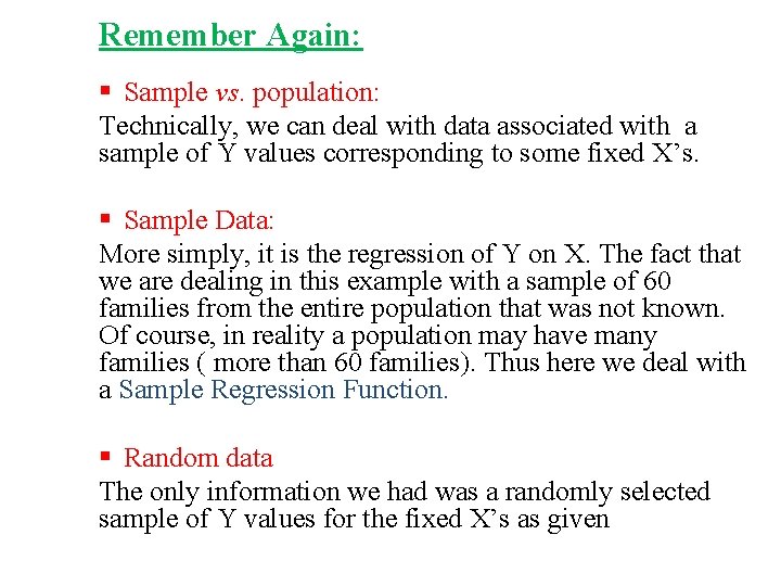
Remember Again: § Sample vs. population: Technically, we can deal with data associated with a sample of Y values corresponding to some fixed X’s. § Sample Data: More simply, it is the regression of Y on X. The fact that we are dealing in this example with a sample of 60 families from the entire population that was not known. Of course, in reality a population may have many families ( more than 60 families). Thus here we deal with a Sample Regression Function. § Random data The only information we had was a randomly selected sample of Y values for the fixed X’s as given

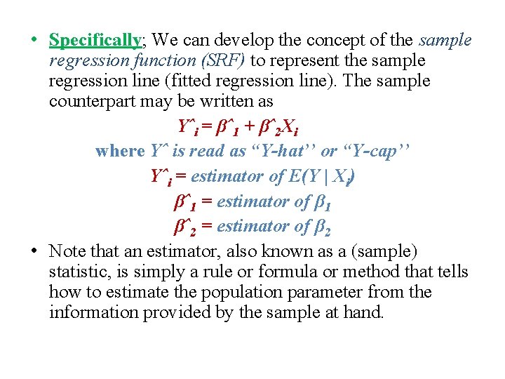
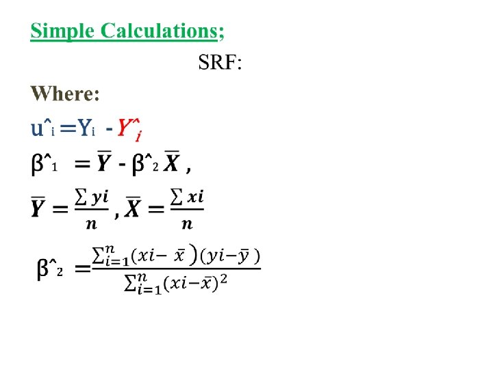
• Specifically; We can develop the concept of the sample regression function (SRF) to represent the sample regression line (fitted regression line). The sample counterpart may be written as Yˆi = βˆ1 + βˆ2 Xi where Yˆ is read as “Y-hat’’ or “Y-cap’’ Yˆi = estimator of E(Y | Xi) βˆ1 = estimator of β 1 βˆ2 = estimator of β 2 • Note that an estimator, also known as a (sample) statistic, is simply a rule or formula or method that tells how to estimate the population parameter from the information provided by the sample at hand.

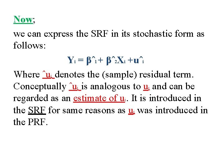
Now; we can express the SRF in its stochastic form as follows: Yi = βˆ1 + βˆ2 Xi +uˆi Where ˆui denotes the (sample) residual term. Conceptually ˆui is analogous to ui and can be regarded as an estimate of ui. It is introduced in the SRF for same reasons as ui was introduced in the PRF.

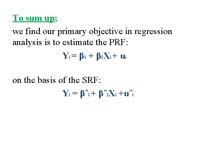
To sum up; we find our primary objective in regression analysis is to estimate the PRF: Yi = β 1 + β 2 Xi + ui on the basis of the SRF: Yi = βˆ1 + βˆ2 Xi +uˆi

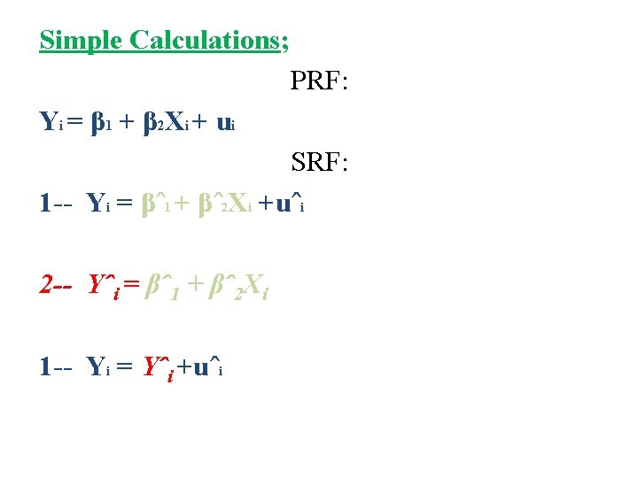
Simple Calculations; PRF: Yi = β 1 + β 2 Xi + ui SRF: 1 -- Yi = βˆ1 + βˆ2 Xi +uˆi 2 -- Yˆi = βˆ1 + βˆ2 Xi 1 -- Yi = Yˆi +uˆi

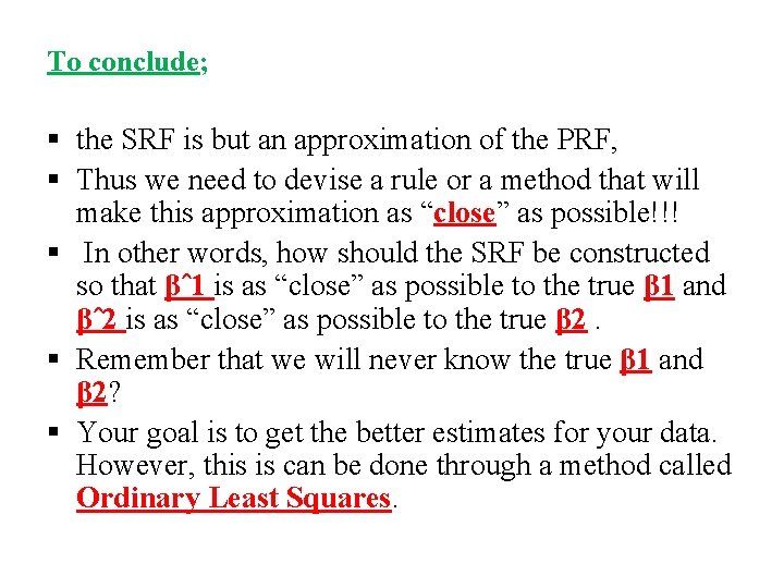
To conclude; § the SRF is but an approximation of the PRF, § Thus we need to devise a rule or a method that will make this approximation as “close” as possible!!! § In other words, how should the SRF be constructed so that βˆ1 is as “close” as possible to the true β 1 and βˆ2 is as “close” as possible to the true β 2. § Remember that we will never know the true β 1 and β 2? § Your goal is to get the better estimates for your data. However, this is can be done through a method called Ordinary Least Squares.