CHAPTER 2 FUNCTIONAL FORMS OF REGRESSION MODELS Damodar

CHAPTER 2 FUNCTIONAL FORMS OF REGRESSION MODELS Damodar Gujarati Econometrics by Example, second edition

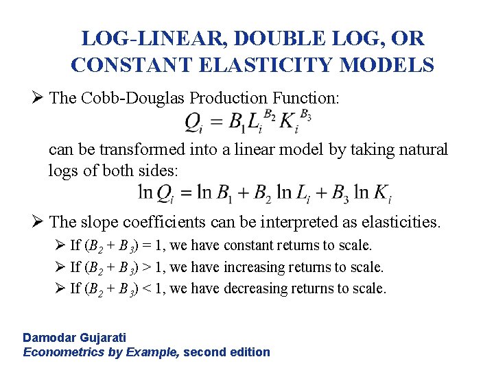
LOG-LINEAR, DOUBLE LOG, OR CONSTANT ELASTICITY MODELS Ø The Cobb-Douglas Production Function: can be transformed into a linear model by taking natural logs of both sides: Ø The slope coefficients can be interpreted as elasticities. Ø If (B 2 + B 3) = 1, we have constant returns to scale. Ø If (B 2 + B 3) > 1, we have increasing returns to scale. Ø If (B 2 + B 3) < 1, we have decreasing returns to scale. Damodar Gujarati Econometrics by Example, second edition

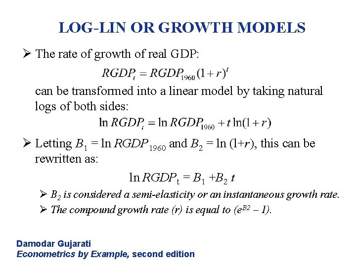
LOG-LIN OR GROWTH MODELS Ø The rate of growth of real GDP: can be transformed into a linear model by taking natural logs of both sides: Ø Letting B 1 = ln RGDP 1960 and B 2 = ln (l+r), this can be rewritten as: ln RGDPt = B 1 +B 2 t Ø B 2 is considered a semi-elasticity or an instantaneous growth rate. Ø The compound growth rate (r) is equal to (e. B 2 – 1). Damodar Gujarati Econometrics by Example, second edition

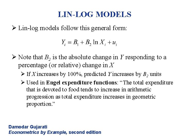
LIN-LOG MODELS Ø Lin-log models follow this general form: Ø Note that B 2 is the absolute change in Y responding to a percentage (or relative) change in X Ø If X increases by 100%, predicted Y increases by B 2 units Ø Used in Engel expenditure functions: “The total expenditure that is devoted to food tends to increase in arithmetic progression as total expenditure increases in geometric proportion. ” Damodar Gujarati Econometrics by Example, second edition

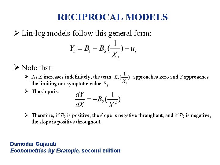
RECIPROCAL MODELS Ø Lin-log models follow this general form: Ø Note that: Ø As X increases indefinitely, the term the limiting or asymptotic value B 1. Ø The slope is: approaches zero and Y approaches Ø Therefore, if B 2 is positive, the slope is negative throughout, and if B 2 is negative, the slope is positive throughout. Damodar Gujarati Econometrics by Example, second edition

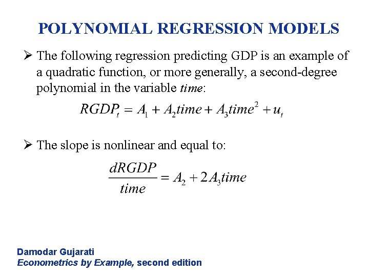
POLYNOMIAL REGRESSION MODELS Ø The following regression predicting GDP is an example of a quadratic function, or more generally, a second-degree polynomial in the variable time: Ø The slope is nonlinear and equal to: Damodar Gujarati Econometrics by Example, second edition

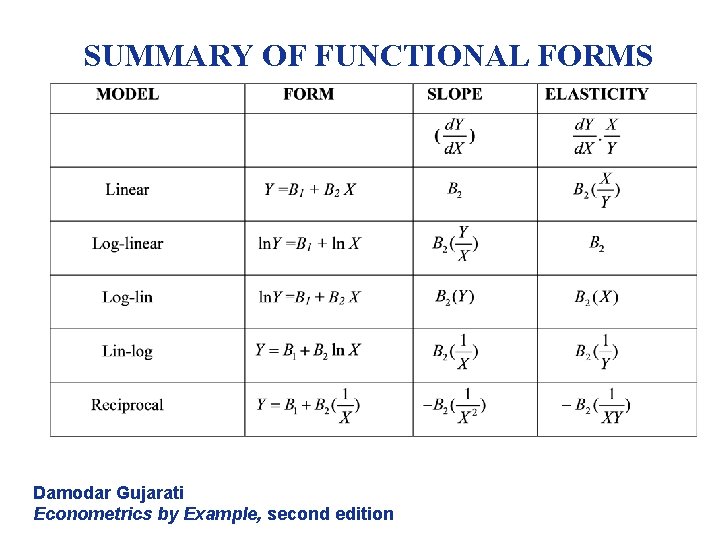
SUMMARY OF FUNCTIONAL FORMS Damodar Gujarati Econometrics by Example, second edition

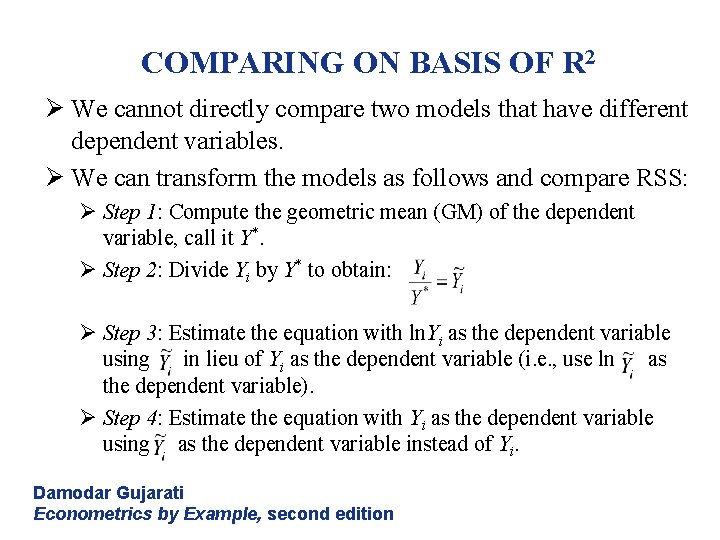
COMPARING ON BASIS OF R 2 Ø We cannot directly compare two models that have different dependent variables. Ø We can transform the models as follows and compare RSS: Ø Step 1: Compute the geometric mean (GM) of the dependent variable, call it Y*. Ø Step 2: Divide Yi by Y* to obtain: Ø Step 3: Estimate the equation with ln. Yi as the dependent variable using in lieu of Yi as the dependent variable (i. e. , use ln as the dependent variable). Ø Step 4: Estimate the equation with Yi as the dependent variable using as the dependent variable instead of Yi. Damodar Gujarati Econometrics by Example, second edition

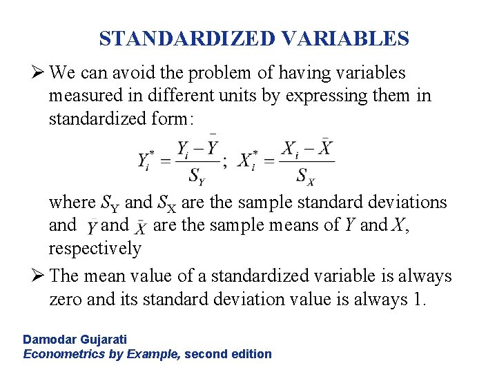
STANDARDIZED VARIABLES Ø We can avoid the problem of having variables measured in different units by expressing them in standardized form: where SY and SX are the sample standard deviations and are the sample means of Y and X, respectively Ø The mean value of a standardized variable is always zero and its standard deviation value is always 1. Damodar Gujarati Econometrics by Example, second edition

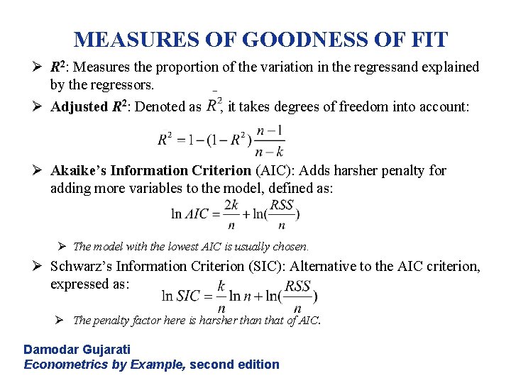
MEASURES OF GOODNESS OF FIT Ø R 2: Measures the proportion of the variation in the regressand explained by the regressors. Ø Adjusted R 2: Denoted as , it takes degrees of freedom into account: Ø Akaike’s Information Criterion (AIC): Adds harsher penalty for adding more variables to the model, defined as: Ø The model with the lowest AIC is usually chosen. Ø Schwarz’s Information Criterion (SIC): Alternative to the AIC criterion, expressed as: Ø The penalty factor here is harsher than that of AIC. Damodar Gujarati Econometrics by Example, second edition

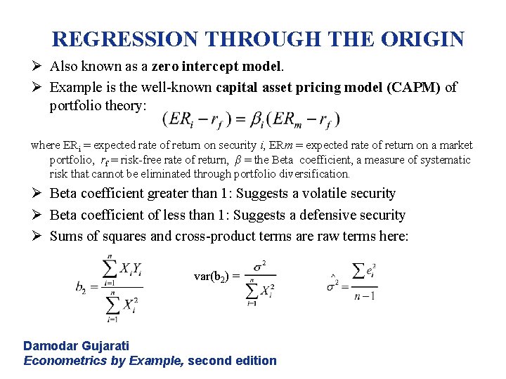
REGRESSION THROUGH THE ORIGIN Ø Also known as a zero intercept model. Ø Example is the well-known capital asset pricing model (CAPM) of portfolio theory: where ERi = expected rate of return on security i, ERm = expected rate of return on a market portfolio, rf = risk-free rate of return, β = the Beta coefficient, a measure of systematic risk that cannot be eliminated through portfolio diversification. Ø Beta coefficient greater than 1: Suggests a volatile security Ø Beta coefficient of less than 1: Suggests a defensive security Ø Sums of squares and cross-product terms are raw terms here: var(b 2) = Damodar Gujarati Econometrics by Example, second edition