Econometrics Lecture 6 GMMEstimator and Econometric Models Contents

Econometrics - Lecture 6 GMM-Estimator and Econometric Models

Contents n n n n The IV Estimator The Generalized Method of Moments The GMM Estimator Econometric Models Dynamic Models Multi-equation Models Jan 7, 2011 Hackl, Econometrics, Lecture 6 2

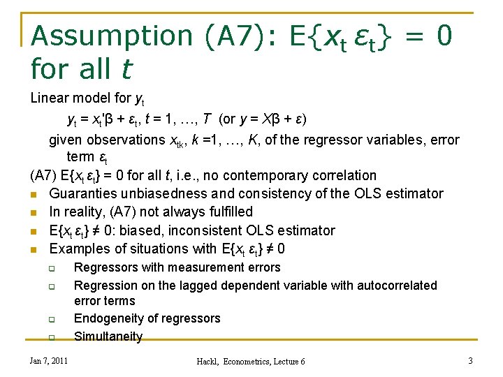
Assumption (A 7): E{xt εt} = 0 for all t Linear model for yt yt = xt'β + εt, t = 1, …, T (or y = Xβ + ε) given observations xtk, k =1, …, K, of the regressor variables, error term εt (A 7) E{xt εt} = 0 for all t, i. e. , no contemporary correlation n Guaranties unbiasedness and consistency of the OLS estimator n In reality, (A 7) not always fulfilled n E{xt εt} ≠ 0: biased, inconsistent OLS estimator n Examples of situations with E{xt εt} ≠ 0 q q Jan 7, 2011 Regressors with measurement errors Regression on the lagged dependent variable with autocorrelated error terms Endogeneity of regressors Simultaneity Hackl, Econometrics, Lecture 6 3

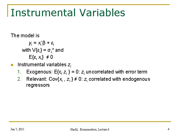
Instrumental Variables The model is yt = xt‘β + εt with V{εi} = σε² and E{εt xt} ≠ 0 n Instrumental variables zt 1. Exogenous: E{εt zt } = 0: zt uncorrelated with error term 2. Relevant: Cov{xt , zt } ≠ 0: zt correlated with endogenous regressors Jan 7, 2011 Hackl, Econometrics, Lecture 6 4

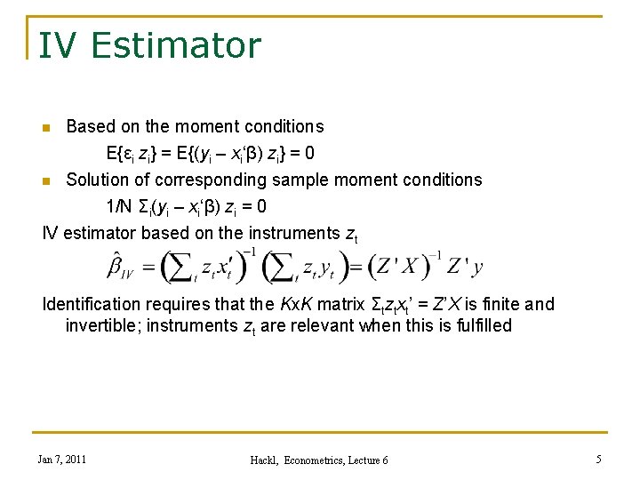
IV Estimator n Based on the moment conditions E{εi zi} = E{(yi – xi‘β) zi} = 0 Solution of corresponding sample moment conditions 1/N Σi(yi – xi‘β) zi = 0 IV estimator based on the instruments zt n Identification requires that the Kx. K matrix Σtztxt’ = Z’X is finite and invertible; instruments zt are relevant when this is fulfilled Jan 7, 2011 Hackl, Econometrics, Lecture 6 5

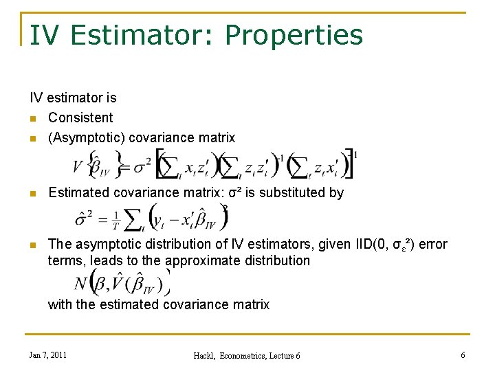
IV Estimator: Properties IV estimator is n Consistent n (Asymptotic) covariance matrix n Estimated covariance matrix: σ² is substituted by n The asymptotic distribution of IV estimators, given IID(0, σε²) error terms, leads to the approximate distribution with the estimated covariance matrix Jan 7, 2011 Hackl, Econometrics, Lecture 6 6

Contents n n n n The IV Estimator The Generalized Method of Moments The GMM Estimator Econometric Models Dynamic Models Multi-equation Models Jan 7, 2011 Hackl, Econometrics, Lecture 6 7

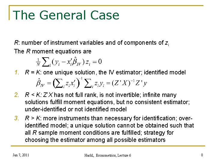
The General Case R: number of instrument variables and of components of zi The R moment equations are 1. R = K: one unique solution, the IV estimator; identified model 2. R < K: Z’X has not full rank, is not invertible; infinite many solutions fulfill moment equations, but no consistent estimator; under-identified or not identified model 3. R > K: more instruments than necessary for identification; overidentified model; a unique solution cannot be obtained such that all R sample moment conditions are fulfilled; strategy for choosing the estimator among all possible estimators Jan 7, 2011 Hackl, Econometrics, Lecture 6 8

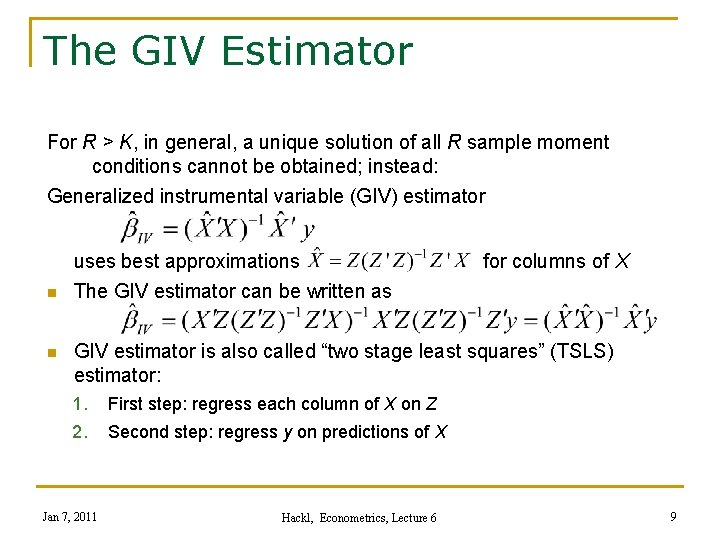
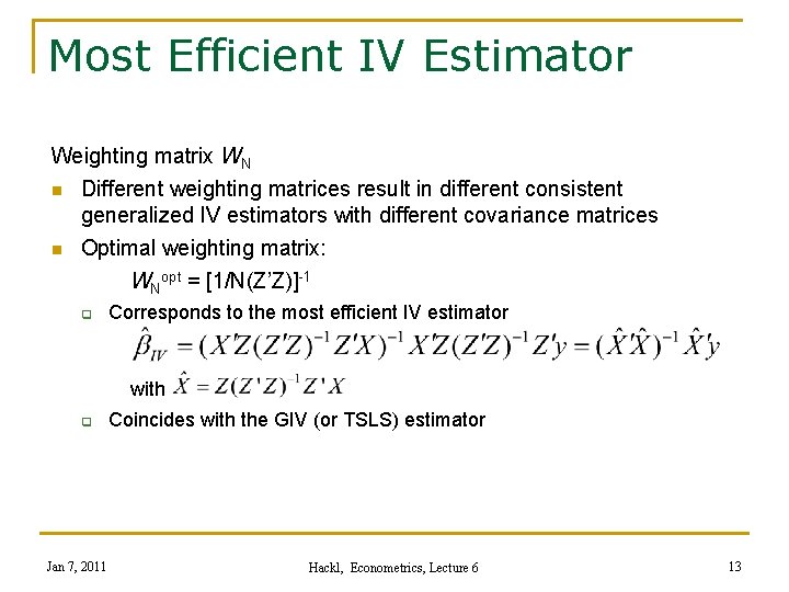
The GIV Estimator For R > K, in general, a unique solution of all R sample moment conditions cannot be obtained; instead: Generalized instrumental variable (GIV) estimator n n uses best approximations for columns of X The GIV estimator can be written as GIV estimator is also called “two stage least squares” (TSLS) estimator: 1. 2. Jan 7, 2011 First step: regress each column of X on Z Second step: regress y on predictions of X Hackl, Econometrics, Lecture 6 9

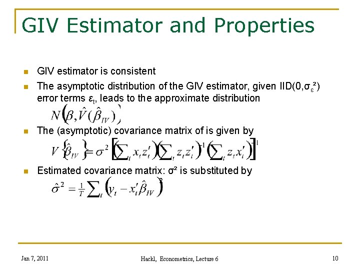
GIV Estimator and Properties n GIV estimator is consistent The asymptotic distribution of the GIV estimator, given IID(0, σε²) error terms εt, leads to the approximate distribution n The (asymptotic) covariance matrix of is given by n Estimated covariance matrix: σ² is substituted by n Jan 7, 2011 Hackl, Econometrics, Lecture 6 10

Contents n n n n The IV Estimator The Generalized Method of Moments The GMM Estimator Econometric Models Dynamic Models Multi-equation Models Jan 7, 2011 Hackl, Econometrics, Lecture 6 11

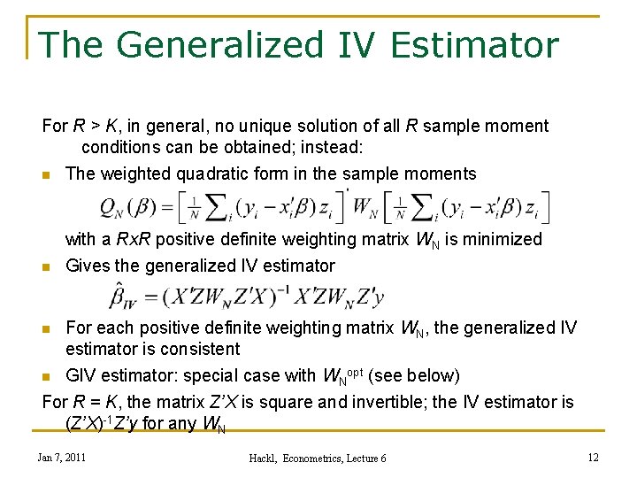
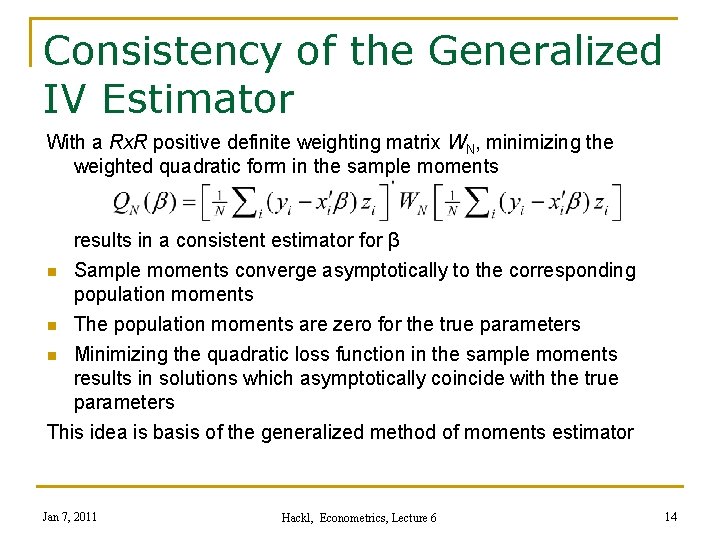
The Generalized IV Estimator For R > K, in general, no unique solution of all R sample moment conditions can be obtained; instead: n The weighted quadratic form in the sample moments n with a Rx. R positive definite weighting matrix WN is minimized Gives the generalized IV estimator For each positive definite weighting matrix WN, the generalized IV estimator is consistent n GIV estimator: special case with WNopt (see below) For R = K, the matrix Z’X is square and invertible; the IV estimator is (Z’X)-1 Z’y for any WN n Jan 7, 2011 Hackl, Econometrics, Lecture 6 12

Most Efficient IV Estimator Weighting matrix WN n Different weighting matrices result in different consistent generalized IV estimators with different covariance matrices n Optimal weighting matrix: WNopt = [1/N(Z’Z)]-1 q Corresponds to the most efficient IV estimator with q Jan 7, 2011 Coincides with the GIV (or TSLS) estimator Hackl, Econometrics, Lecture 6 13

Consistency of the Generalized IV Estimator With a Rx. R positive definite weighting matrix WN, minimizing the weighted quadratic form in the sample moments results in a consistent estimator for β n Sample moments converge asymptotically to the corresponding population moments n The population moments are zero for the true parameters n Minimizing the quadratic loss function in the sample moments results in solutions which asymptotically coincide with the true parameters This idea is basis of the generalized method of moments estimator Jan 7, 2011 Hackl, Econometrics, Lecture 6 14

Generalized Method of Moments (GMM) Estimator n n n GMM generalizes the IV estimation concept Estimates of model parameters are derived from moment conditions which are not necessarily linear Number of moment conditions at least as large as number of unknown parameters Jan 7, 2011 Hackl, Econometrics, Lecture 6 15

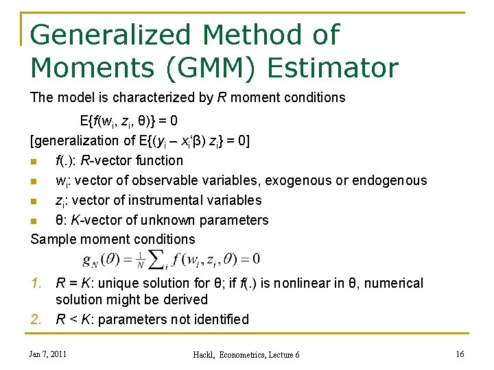
Generalized Method of Moments (GMM) Estimator The model is characterized by R moment conditions E{f(wi, zi, θ)} = 0 [generalization of E{(yi – xi‘β) zi} = 0] n f(. ): R-vector function n wi: vector of observable variables, exogenous or endogenous n zi: vector of instrumental variables n θ: K-vector of unknown parameters Sample moment conditions 1. R = K: unique solution for θ; if f(. ) is nonlinear in θ, numerical solution might be derived 2. R < K: parameters not identified Jan 7, 2011 Hackl, Econometrics, Lecture 6 16

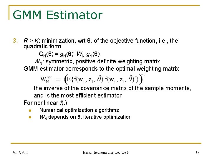
GMM Estimator 3. R > K: minimization, wrt θ, of the objective function, i. e. , the quadratic form QN(θ) = g. N(θ)‘ WN g. N(θ) WN: symmetric, positive definite weighting matrix GMM estimator corresponds to the optimal weighting matrix the inverse of the covariance matrix of the sample moments, and is the most efficient estimator For nonlinear f(. ) n n Jan 7, 2011 Numerical optimization algorithms WN depends on θ; iterative optimization Hackl, Econometrics, Lecture 6 17

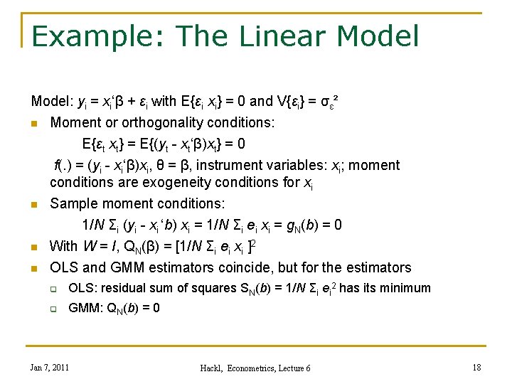
Example: The Linear Model: yi = xi‘β + εi with E{εi xi} = 0 and V{εi} = σε² n Moment or orthogonality conditions: n n n E{εt xt} = E{(yt - xt‘β)xt} = 0 f(. ) = (yi - xi‘β)xi, θ = β, instrument variables: xi; moment conditions are exogeneity conditions for xi Sample moment conditions: 1/N Σi (yi - xi ‘b) xi = 1/N Σi ei xi = g. N(b) = 0 With W = I, QN(β) = [1/N Σi ei xi ]2 OLS and GMM estimators coincide, but for the estimators q OLS: residual sum of squares SN(b) = 1/N Σi ei 2 has its minimum q GMM: QN(b) = 0 Jan 7, 2011 Hackl, Econometrics, Lecture 6 18

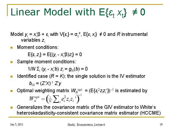
Linear Model with E{εt xt} ≠ 0 Model yi = xi‘β + εi with V{εi} = σε², E{εi xi} ≠ 0 and R instrumental variables zi n n n Moment conditions: E{εi zi} = E{(yi - xi‘β)zi} = 0 Sample moment conditions: 1/N Σi (yi - xi‘b) zi = g. N(b) = 0 Identified case (R = K): the single solution is the IV estimator b. IV = (Z’X)-1 Z’y Optimal weighting matrix WNopt = (E{εi 2 zizi‘}) -1 is estimated by Generalizes the covariance matrix of the GIV estimator to White‘s heteroskedasticity-consistent covariance matrix estimator (HCCME) Jan 7, 2011 Hackl, Econometrics, Lecture 6 19

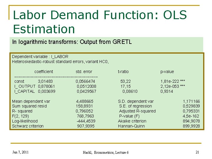
Example: Labor Demand Verbeek’s data set “labour 2”: Sample of 569 Belgian companies (data from 1996) n n Variables q labour: total employment (number of employees) q capital: total fixed assets q wage: total wage costs per employee (in 1000 EUR) q output: value added (in million EUR) Labour demand function labour = b 1 + b 2*output + b 3*capital Jan 7, 2011 Hackl, Econometrics, Lecture 6 20

Labor Demand Function: OLS Estimation In logarithmic transforms: Output from GRETL Dependent variable : l_LABOR Heteroskedastic-robust standard errors, variant HC 0, coefficient std. error ------------------------------ const 3, 01483 0, 0566474 l_ OUTPUT 0, 878061 0, 0512008 l_CAPITAL 0, 003699 0, 0429567 t-ratio p-value 53, 22 17, 15 0, 08610 1, 81 e-222 *** 2, 12 e-053 *** 0, 9314 Mean dependent var 4, 488665 Sum squared resid 158, 8931 R- squared 0, 796052 F(2, 129) 768, 7963 Log-likelihood -444, 4539 Schwarz criterion 907, 9395 S. D. dependent var S. E. of regression Adjusted R-squared P-value (F) Akaike criterion Hannan-Quinn Jan 7, 2011 Hackl, Econometrics, Lecture 6 1, 171166 0, 529839 0, 795331 4, 5 e-162 894, 9078 899, 9928 21

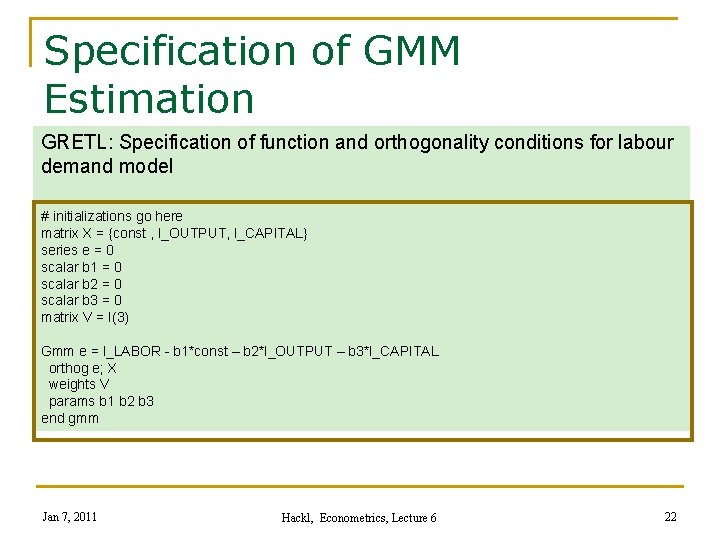
Specification of GMM Estimation GRETL: Specification of function and orthogonality conditions for labour demand model # initializations go here matrix X = {const , l_OUTPUT, l_CAPITAL} series e = 0 scalar b 1 = 0 scalar b 2 = 0 scalar b 3 = 0 matrix V = I(3) Gmm e = l_LABOR - b 1*const – b 2*l_OUTPUT – b 3*l_CAPITAL orthog e; X weights V params b 1 b 2 b 3 end gmm Jan 7, 2011 Hackl, Econometrics, Lecture 6 22

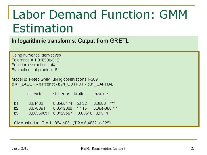
Labor Demand Function: GMM Estimation In logarithmic transforms: Output from GRETL Using numerical derivatives Tolerance = 1, 81899 e-012 Function evaluations: 44 Evaluations of gradient: 8 Model 8: 1 -step GMM, using observations 1 -569 e = l_LABOR - b 1*const - b 2*l_OUTPUT - b 3*l_CAPITAL estimate std. error t-ratio p-value ------------------------------------- b 1 3, 01483 0, 0566474 53, 22 0, 0000 *** b 2 0, 878061 0, 0512008 17, 15 6, 36 e-066 *** b 3 0, 00369851 0, 0429567 0, 08610 0, 9314 GMM criterion: Q = 1, 1394 e-031 (TQ = 6, 48321 e-029) Jan 7, 2011 Hackl, Econometrics, Lecture 6 23

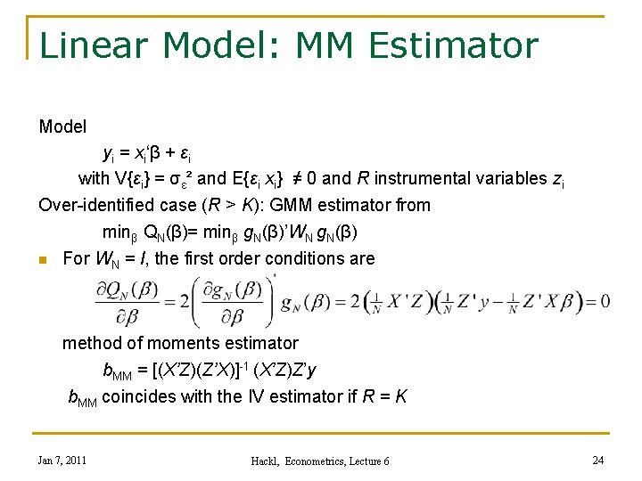
Linear Model: MM Estimator Model yi = xi‘β + εi with V{εi} = σε² and E{εi xi} ≠ 0 and R instrumental variables zi Over-identified case (R > K): GMM estimator from minβ QN(β)= minβ g. N(β)’WN g. N(β) n For WN = I, the first order conditions are method of moments estimator b. MM = [(X’Z)(Z’X)]-1 (X’Z)Z’y b. MM coincides with the IV estimator if R = K Jan 7, 2011 Hackl, Econometrics, Lecture 6 24

Contents n n n n The IV Estimator The Generalized Method of Moments The GMM Estimator Econometric Models Dynamic Models Multi-equation Models Jan 7, 2011 Hackl, Econometrics, Lecture 6 25

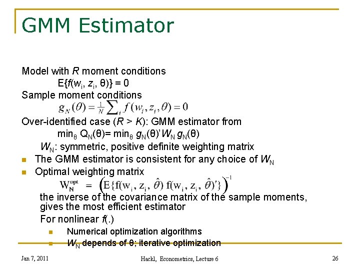
GMM Estimator Model with R moment conditions E{f(wi, zi, θ)} = 0 Sample moment conditions Over-identified case (R > K): GMM estimator from minθ QN(θ)= minθ g. N(θ)’WN g. N(θ) WN: symmetric, positive definite weighting matrix n The GMM estimator is consistent for any choice of WN n Optimal weighting matrix the inverse of the covariance matrix of the sample moments, gives the most efficient estimator For nonlinear f(. ) n n Jan 7, 2011 Numerical optimization algorithms WN depends of θ; iterative optimization Hackl, Econometrics, Lecture 6 26

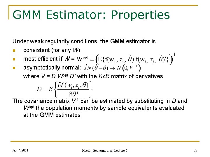
GMM Estimator: Properties Under weak regularity conditions, the GMM estimator is n consistent (for any W) n n most efficient if W = asymptotically normal: where V = D Wopt D’ with the Kx. R matrix of derivatives The covariance matrix V-1 can be estimated by substituting in D and Wopt the population moments by sample equivalents evaluated at the GMM estimates Jan 7, 2011 Hackl, Econometrics, Lecture 6 27

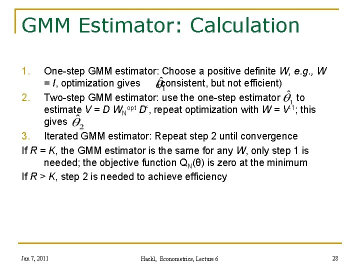
GMM Estimator: Calculation 1. One-step GMM estimator: Choose a positive definite W, e. g. , W = I, optimization gives (consistent, but not efficient) 2. Two-step GMM estimator: use the one-step estimator to estimate V = D WNopt D‘, repeat optimization with W = V-1; this gives 3. Iterated GMM estimator: Repeat step 2 until convergence If R = K, the GMM estimator is the same for any W, only step 1 is needed; the objective function QN(θ) is zero at the minimum If R > K, step 2 is needed to achieve efficiency Jan 7, 2011 Hackl, Econometrics, Lecture 6 28

Contents n n n n The IV Estimator The Generalized Method of Moments The GMM Estimator Econometric Models Dynamic Models Multi-equation Models Jan 7, 2011 Hackl, Econometrics, Lecture 6 29

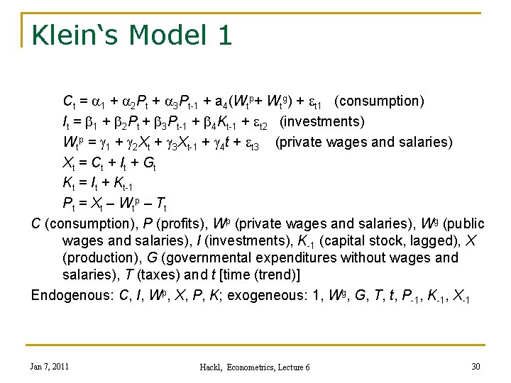
Klein‘s Model 1 Ct = a 1 + a 2 Pt + a 3 Pt-1 + a 4(Wtp+ Wtg) + et 1 (consumption) It = b 1 + b 2 Pt + b 3 Pt-1 + b 4 Kt-1 + et 2 (investments) Wtp = g 1 + g 2 Xt + g 3 Xt-1 + g 4 t + et 3 (private wages and salaries) Xt = Ct + It + Gt Kt = It + Kt-1 Pt = Xt – Wtp – Tt C (consumption), P (profits), Wp (private wages and salaries), Wg (public wages and salaries), I (investments), K-1 (capital stock, lagged), X (production), G (governmental expenditures without wages and salaries), T (taxes) and t [time (trend)] Endogenous: C, I, Wp, X, P, K; exogeneous: 1, Wg, G, T, t, P-1, K-1, X-1 Jan 7, 2011 Hackl, Econometrics, Lecture 6 30

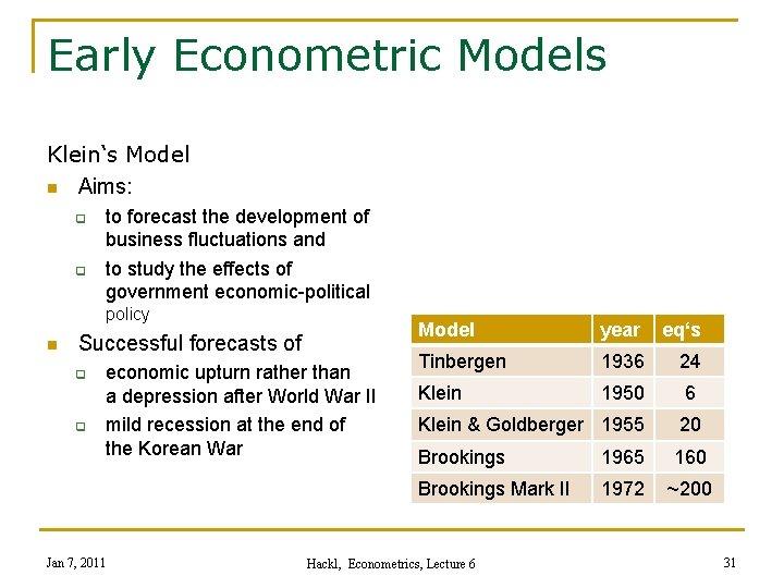
Early Econometric Models Klein‘s Model n Aims: q q to forecast the development of business fluctuations and to study the effects of government economic-political policy n Successful forecasts of q q economic upturn rather than a depression after World War II mild recession at the end of the Korean War Jan 7, 2011 Model year eq‘s Tinbergen 1936 24 Klein 1950 6 Klein & Goldberger 1955 20 Brookings 1965 160 Brookings Mark II 1972 ~200 Hackl, Econometrics, Lecture 6 31

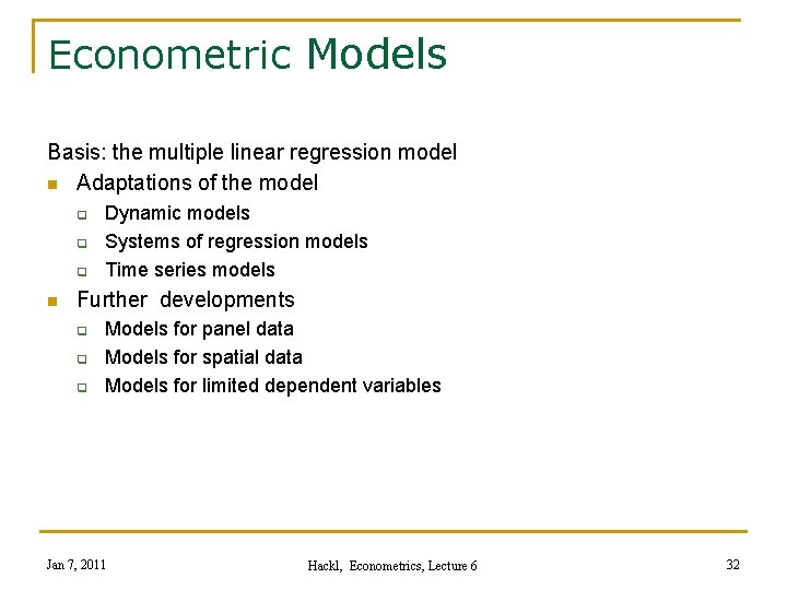
Econometric Models Basis: the multiple linear regression model n Adaptations of the model q q q n Dynamic models Systems of regression models Time series models Further developments q q q Models for panel data Models for spatial data Models for limited dependent variables Jan 7, 2011 Hackl, Econometrics, Lecture 6 32

Contents n n n n The IV Estimator The Generalized Method of Moments The GMM Estimator Econometric Models Dynamic Models Multi-equation Models Jan 7, 2011 Hackl, Econometrics, Lecture 6 33

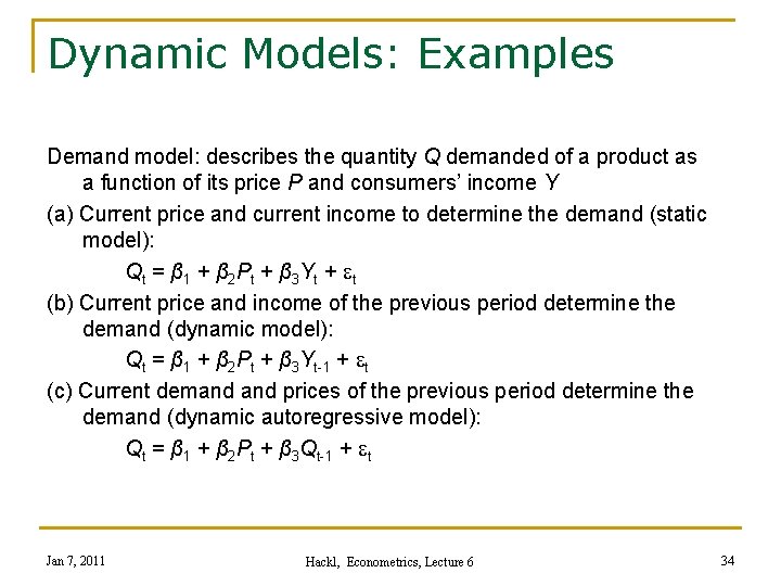
Dynamic Models: Examples Demand model: describes the quantity Q demanded of a product as a function of its price P and consumers’ income Y (a) Current price and current income to determine the demand (static model): Qt = β 1 + β 2 Pt + β 3 Yt + et (b) Current price and income of the previous period determine the demand (dynamic model): Qt = β 1 + β 2 Pt + β 3 Yt-1 + et (c) Current demand prices of the previous period determine the demand (dynamic autoregressive model): Qt = β 1 + β 2 Pt + β 3 Qt-1 + et Jan 7, 2011 Hackl, Econometrics, Lecture 6 34

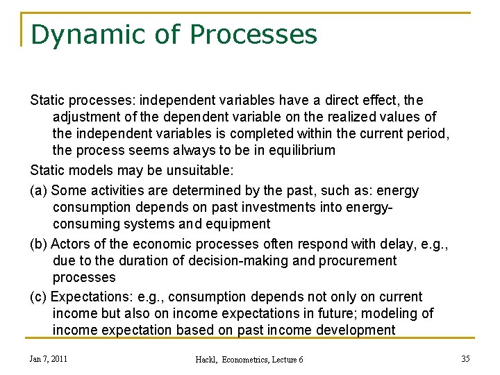
Dynamic of Processes Static processes: independent variables have a direct effect, the adjustment of the dependent variable on the realized values of the independent variables is completed within the current period, the process seems always to be in equilibrium Static models may be unsuitable: (a) Some activities are determined by the past, such as: energy consumption depends on past investments into energyconsuming systems and equipment (b) Actors of the economic processes often respond with delay, e. g. , due to the duration of decision-making and procurement processes (c) Expectations: e. g. , consumption depends not only on current income but also on income expectations in future; modeling of income expectation based on past income development Jan 7, 2011 Hackl, Econometrics, Lecture 6 35

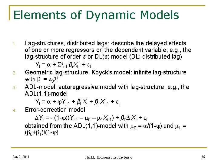
Elements of Dynamic Models 1. 2. 3. 4. Lag-structures, distributed lags: describe the delayed effects of one or more regressors on the dependent variable; e. g. , the lag-structure of order s or DL(s) model (DL: distributed lag) Yt = a + Ssi=0βi. Xt-i + et Geometric lag-structure, Koyck’s model: infinite lag-structure with bi = l 0 li ADL-model: autoregressive model with lag-structure, e. g. , the ADL(1, 1)-model Yt = a + j. Yt-1 + β 0 Xt + β 1 Xt-1 + et Error-correction model DYt = - (1 -j)(Yt-1 – m 0 – m 1 Xt-1) + β 0 D Xt + et obtained from the ADL(1, 1)-model with m 0 = a/(1 -j) und m 1 = (b 0+b 1)/(1 -j) Jan 7, 2011 Hackl, Econometrics, Lecture 6 36

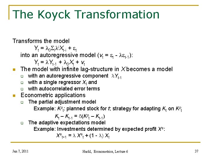
The Koyck Transformation Transforms the model Yt = l 0 Sili. Xt-i + et into an autoregressive model (vt = et - let-1): Yt = l. Yt-1 + l 0 Xt + vt n The model with infinite lag-structure in X becomes a model q q q n with an autoregressive component l. Yt-1 with a single regressor Xt and with autocorrelated error terms Econometric applications q q The partial adjustment model Example: Kpt: planned stock for t; strategy for adapting Kt on Kpt Kt – Kt-1 = d(Kpt – Kt-1) The adaptive expectations model Example: Investments determined by expected profit Xe: Xet+1 = l Xet + (1 - l) Xt Jan 7, 2011 Hackl, Econometrics, Lecture 6 37

Contents n n n n The IV Estimator The Generalized Method of Moments The GMM Estimator Econometric Models Dynamic Models Multi-equation Models Jan 7, 2011 Hackl, Econometrics, Lecture 6 38

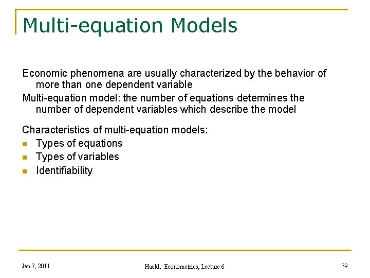
Multi-equation Models Economic phenomena are usually characterized by the behavior of more than one dependent variable Multi-equation model: the number of equations determines the number of dependent variables which describe the model Characteristics of multi-equation models: n Types of equations n Types of variables n Identifiability Jan 7, 2011 Hackl, Econometrics, Lecture 6 39

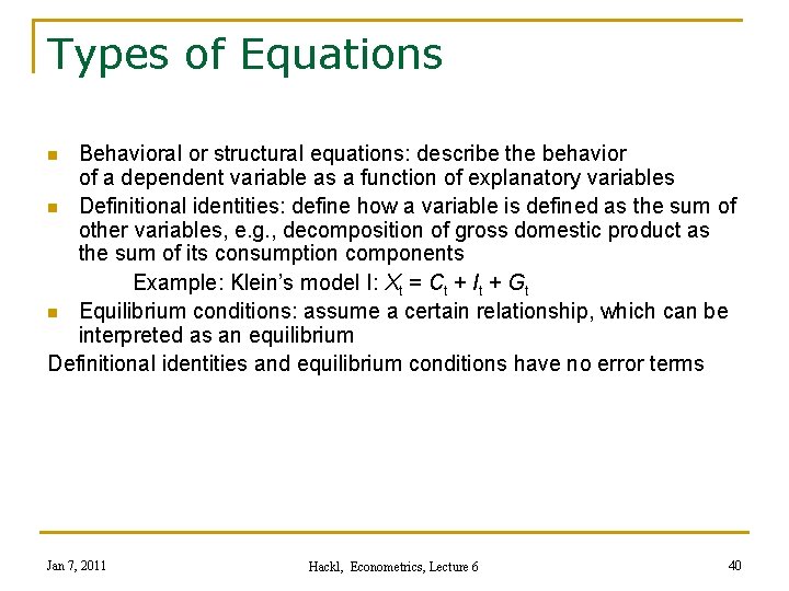
Types of Equations Behavioral or structural equations: describe the behavior of a dependent variable as a function of explanatory variables n Definitional identities: define how a variable is defined as the sum of other variables, e. g. , decomposition of gross domestic product as the sum of its consumption components Example: Klein’s model I: Xt = Ct + It + Gt n Equilibrium conditions: assume a certain relationship, which can be interpreted as an equilibrium Definitional identities and equilibrium conditions have no error terms n Jan 7, 2011 Hackl, Econometrics, Lecture 6 40

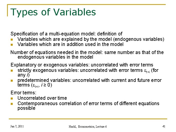
Types of Variables Specification of a multi-equation model: definition of n Variables which are explained by the model (endogenous variables) n Variables which are in addition used in the model Number of equations needed in the model: same number as that of the endogenous variables in the model Explanatory or exogenous variables: uncorrelated with error terms n strictly exogenous variables: uncorrelated with error terms et+i (for any i) n predetermined variables: uncorrelated with current and future error terms (et+i, i ≥ 0) Error terms: n Uncorrelated over time n Contemporaneous correlation of error terms of different equations possible Jan 7, 2011 Hackl, Econometrics, Lecture 6 41

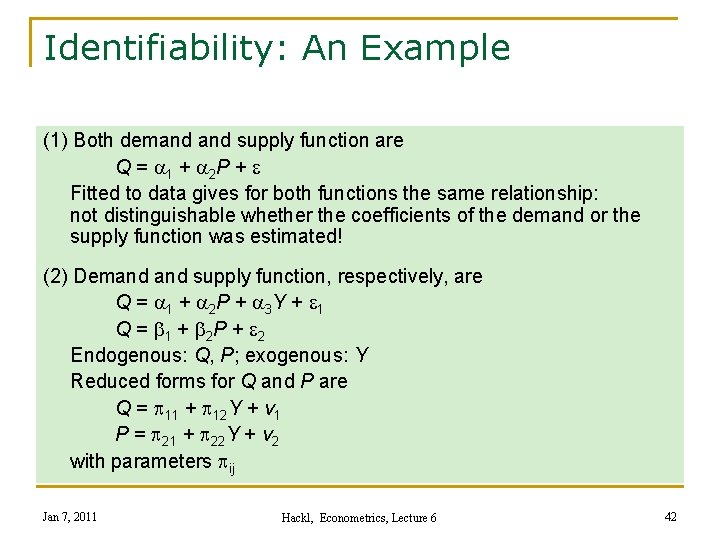
Identifiability: An Example (1) Both demand supply function are Q = a 1 + a 2 P + e Fitted to data gives for both functions the same relationship: not distinguishable whether the coefficients of the demand or the supply function was estimated! (2) Demand supply function, respectively, are Q = a 1 + a 2 P + a 3 Y + e 1 Q = b 1 + b 2 P + e 2 Endogenous: Q, P; exogenous: Y Reduced forms for Q and P are Q = p 11 + p 12 Y + v 1 P = p 21 + p 22 Y + v 2 with parameters pij Jan 7, 2011 Hackl, Econometrics, Lecture 6 42

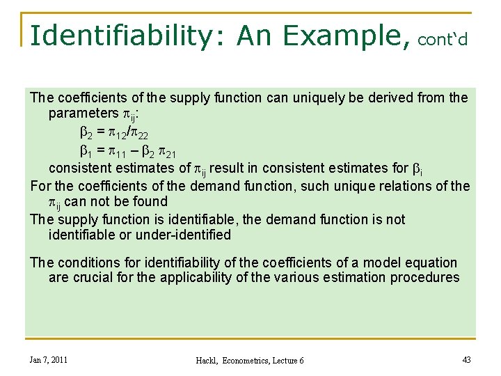
Identifiability: An Example, cont‘d The coefficients of the supply function can uniquely be derived from the parameters pij: b 2 = p 12/p 22 b 1 = p 11 – b 2 p 21 consistent estimates of pij result in consistent estimates for bi For the coefficients of the demand function, such unique relations of the pij can not be found The supply function is identifiable, the demand function is not identifiable or under-identified The conditions for identifiability of the coefficients of a model equation are crucial for the applicability of the various estimation procedures Jan 7, 2011 Hackl, Econometrics, Lecture 6 43

Econometrics II 1. 2. 3. 4. 5. 6. ML Estimation and Specification Tests (MV, Ch. 6) Models with Limited Dependent Variables (MV, Ch. 7) Univariate time series models (MV, Ch. 8) Multivariate time series models, part 1 (MV, Ch. 9) Multivariate time series models, part 2 (MV, Ch. 9) Models Based on Panel Data (MV, Ch. 10) Jan 7, 2011 Hackl, Econometrics, Lecture 6 44