Econometrics Lecture 4 Heteroskedasticity and Autocorrelation Contents n

Econometrics - Lecture 4 Heteroskedasticity and Autocorrelation

Contents n n Violations of V{ε} = s 2 IN Heteroskedasticity GLS Estimation Autocorrelation Nov 12, 2010 Hackl, Econometrics, Lecture 4 2

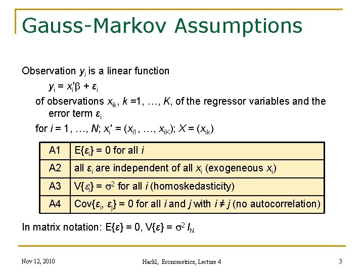
Gauss-Markov Assumptions Observation yi is a linear function yi = xi'b + εi of observations xik, k =1, …, K, of the regressor variables and the error term εi for i = 1, …, N; xi' = (xi 1, …, xi. K); X = (xik) A 1 E{εi} = 0 for all i A 2 all εi are independent of all xi (exogeneous xi) A 3 V{ei} = s 2 for all i (homoskedasticity) A 4 Cov{εi, εj} = 0 for all i and j with i ≠ j (no autocorrelation) In matrix notation: E{ε} = 0, V{ε} = s 2 IN Nov 12, 2010 Hackl, Econometrics, Lecture 4 3

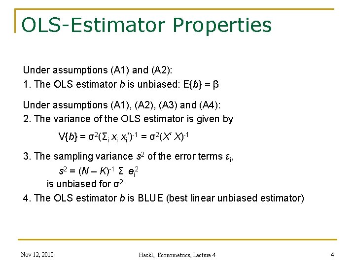
OLS-Estimator Properties Under assumptions (A 1) and (A 2): 1. The OLS estimator b is unbiased: E{b} = β Under assumptions (A 1), (A 2), (A 3) and (A 4): 2. The variance of the OLS estimator is given by V{b} = σ2(Σi xi xi’)-1 = σ2(X‘ X)-1 3. The sampling variance s 2 of the error terms εi, s 2 = (N – K)-1 Σi ei 2 is unbiased for σ2 4. The OLS estimator b is BLUE (best linear unbiased estimator) Nov 12, 2010 Hackl, Econometrics, Lecture 4 4

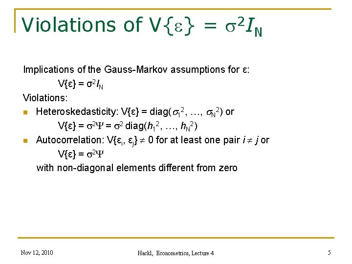
Violations of V{e} = s 2 IN Implications of the Gauss-Markov assumptions for ε: V{ε} = σ2 IN Violations: n Heteroskedasticity: V{ε} = diag(s 12, …, s. N 2) or V{ε} = s 2 Y = s 2 diag(h 12, …, h. N 2) n Autocorrelation: V{εi, εj} 0 for at least one pair i j or V{ε} = s 2 Y with non-diagonal elements different from zero Nov 12, 2010 Hackl, Econometrics, Lecture 4 5

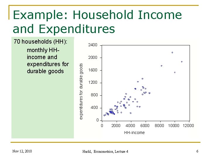
Example: Household Income and Expenditures 2400 2000 expentidures for durable goods 70 households (HH): monthly HHincome and expenditures for durable goods 1600 1200 800 400 0 0 2000 4000 6000 8000 10000 12000 HH-income Nov 12, 2010 Hackl, Econometrics, Lecture 4 6

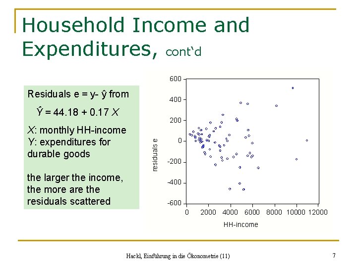
Household Income and Expenditures, cont‘d 600 Residuals e = y- ŷ from 400 Ŷ = 44. 18 + 0. 17 X the larger the income, the more are the residuals scattered residuals e X: monthly HH-income Y: expenditures for durable goods 200 0 -200 -400 -600 0 2000 4000 6000 8000 10000 12000 HH-income Hackl, Einführung in die Ökonometrie (11) 7

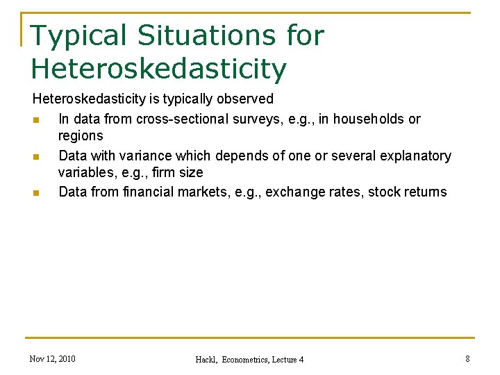
Typical Situations for Heteroskedasticity is typically observed n In data from cross-sectional surveys, e. g. , in households or regions n Data with variance which depends of one or several explanatory variables, e. g. , firm size n Data from financial markets, e. g. , exchange rates, stock returns Nov 12, 2010 Hackl, Econometrics, Lecture 4 8

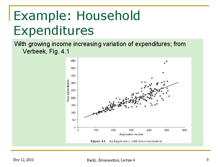
Example: Household Expenditures With growing income increasing variation of expenditures; from Verbeek, Fig. 4. 1 Nov 12, 2010 Hackl, Econometrics, Lecture 4 9

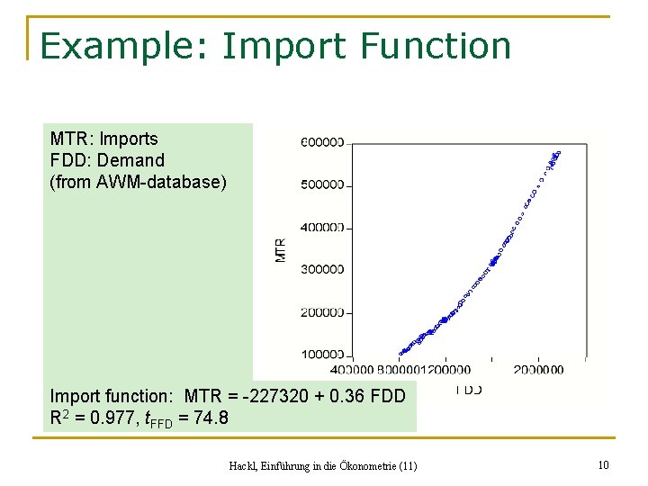
Example: Import Function MTR: Imports FDD: Demand (from AWM-database) Import function: MTR = -227320 + 0. 36 FDD R 2 = 0. 977, t. FFD = 74. 8 Hackl, Einführung in die Ökonometrie (11) 10

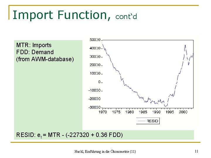
Import Function, cont‘d MTR: Imports FDD: Demand (from AWM-database) RESID: et = MTR - (-227320 + 0. 36 FDD) Hackl, Einführung in die Ökonometrie (11) 11

Import Function, cont‘d Scatter-diagram of by one period lagged residuals [Resid(-1)] against actual residuals [Resid] Serial correlation! Hackl, Einführung in die Ökonometrie (11) 12

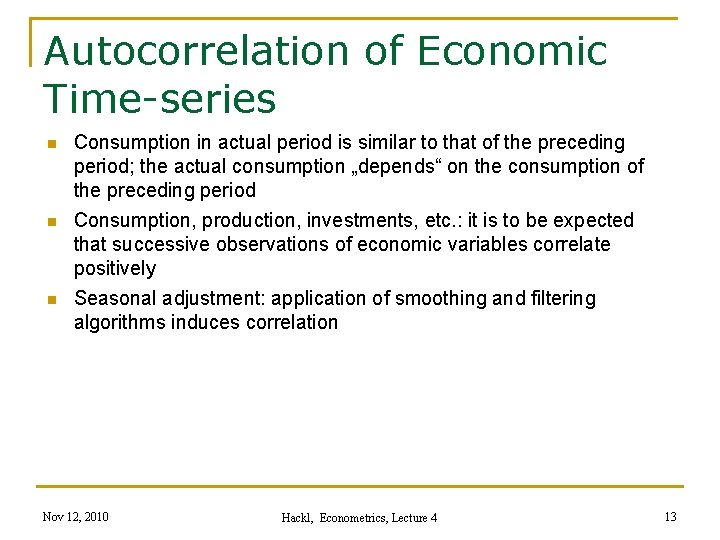
Autocorrelation of Economic Time-series n n n Consumption in actual period is similar to that of the preceding period; the actual consumption „depends“ on the consumption of the preceding period Consumption, production, investments, etc. : it is to be expected that successive observations of economic variables correlate positively Seasonal adjustment: application of smoothing and filtering algorithms induces correlation Nov 12, 2010 Hackl, Econometrics, Lecture 4 13

Example: Imports Scatter-diagram of by one period lagged imports [MTR(-1)] against actual imports [MTR] Correlation coefficient between MTR und MTR( -1): 0. 9994 Hackl, Einführung in die Ökonometrie (11) 14

Typical Situations for Autocorrelation is typically observed if n a relevant regressor with trend or seasonal pattern is not included in the model: miss-specified model n the functional form of a regressor is incorrectly specified n the dependent variable is correlated in a way that is not appropriately represented in the systematic part of the model Warning! Omission of a relevant regressor with trend implies autocorrelation of the error terms; in econometric analyses autocorrelation of the error terms is always possible! n n Autocorrelation of the error terms indicates deficiencies of the model specification Tests for autocorrelation are the most frequently used tool for diagnostic checking the model specification Nov 12, 2010 Hackl, Econometrics, Lecture 4 15

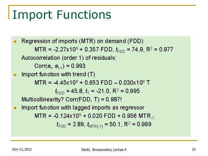
Import Functions n n n Regression of imports (MTR) on demand (FDD) MTR = -2. 27 x 109 + 0. 357 FDD, t. FDD = 74. 9, R 2 = 0. 977 Autocorrelation (order 1) of residuals: Corr(et, et-1) = 0. 993 Import function with trend (T) MTR = -4. 45 x 109 + 0. 653 FDD – 0. 030 x 109 T t. FDD = 45. 8, t. T = -21. 0, R 2 = 0. 995 Multicollinearity? Corr(FDD, T) = 0. 987! Import function with lagged imports as regressor MTR = -0. 124 x 109 + 0. 020 FDD + 0. 956 MTR-1 t. FDD = 2. 89, t. MTR(-1) = 50. 1, R 2 = 0. 999 Nov 12, 2010 Hackl, Econometrics, Lecture 4 16

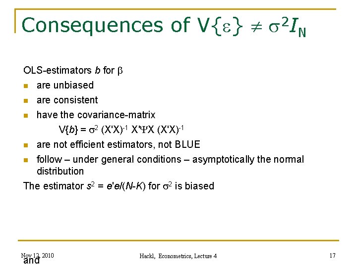
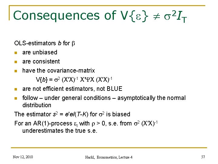
Consequences of V{e} s 2 IN OLS-estimators b for b n are unbiased are consistent n have the covariance-matrix V{b} = s 2 (X'X)-1 X'YX (X'X)-1 n are not efficient estimators, not BLUE n follow – under general conditions – asymptotically the normal distribution The estimator s 2 = e'e/(N-K) for s 2 is biased n Nov 12, 2010 and Hackl, Econometrics, Lecture 4 17

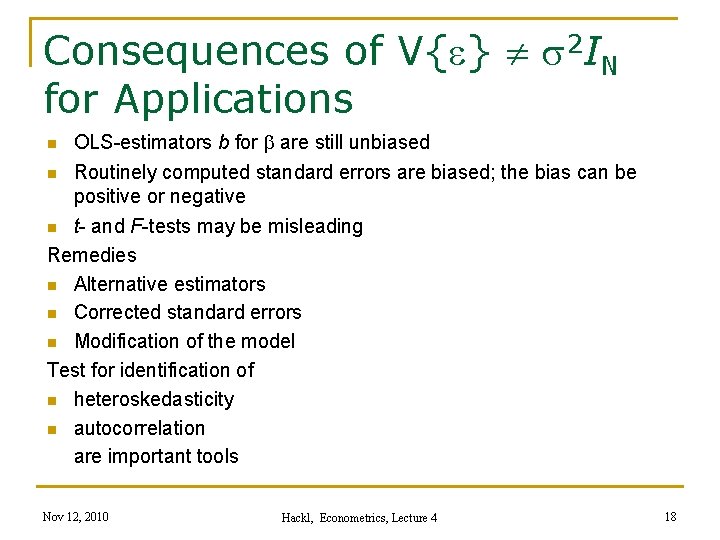
Consequences of V{e} s 2 IN for Applications OLS-estimators b for b are still unbiased n Routinely computed standard errors are biased; the bias can be positive or negative n t- and F-tests may be misleading Remedies n Alternative estimators n Corrected standard errors n Modification of the model Test for identification of n heteroskedasticity n autocorrelation are important tools n Nov 12, 2010 Hackl, Econometrics, Lecture 4 18

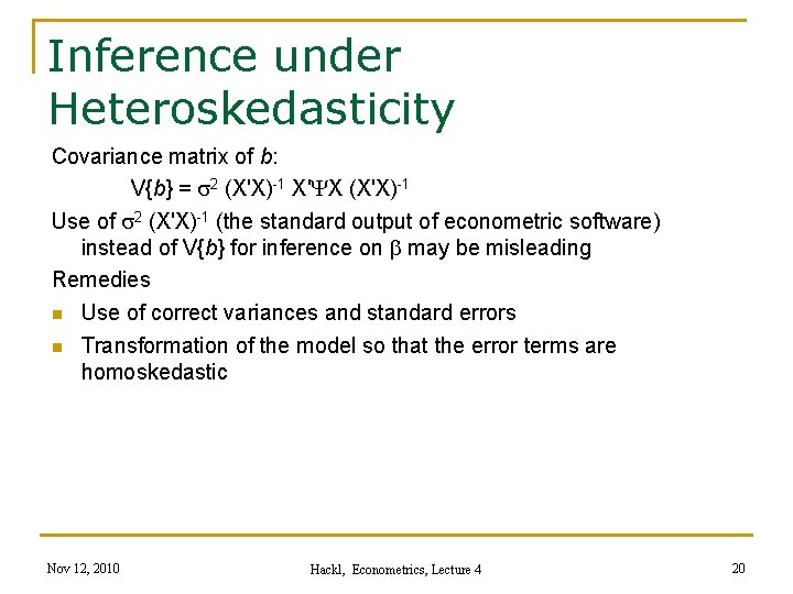
Contents n n Violations of V{ε} = s 2 IN Heteroskedasticity GLS Estimation Autocorrelation Nov 12, 2010 Hackl, Econometrics, Lecture 4 19

Inference under Heteroskedasticity Covariance matrix of b: V{b} = s 2 (X'X)-1 X'YX (X'X)-1 Use of s 2 (X'X)-1 (the standard output of econometric software) instead of V{b} for inference on b may be misleading Remedies n Use of correct variances and standard errors n Transformation of the model so that the error terms are homoskedastic Nov 12, 2010 Hackl, Econometrics, Lecture 4 20

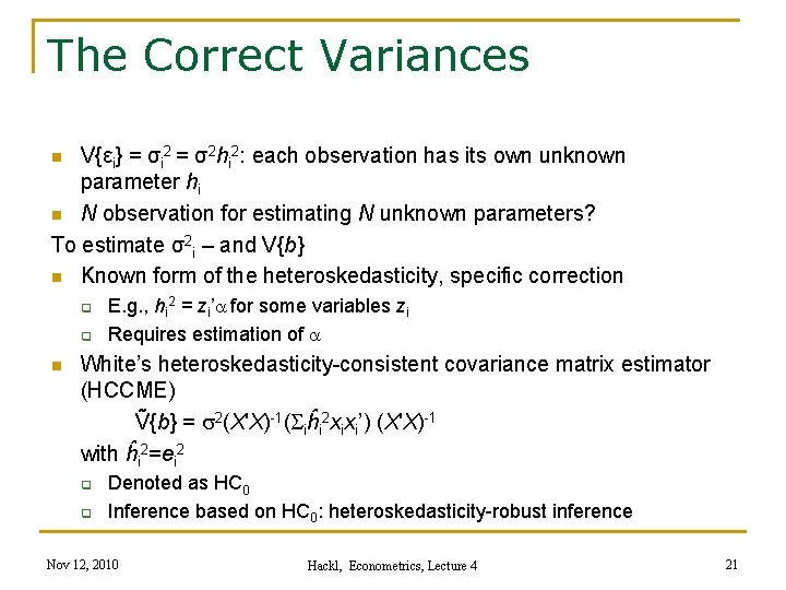
The Correct Variances V{εi} = σi 2 = σ2 hi 2: each observation has its own unknown parameter hi n N observation for estimating N unknown parameters? To estimate σ2 i – and V{b} n Known form of the heteroskedasticity, specific correction n q q n E. g. , hi 2 = zi’a for some variables zi Requires estimation of a White’s heteroskedasticity-consistent covariance matrix estimator (HCCME) Ṽ{b} = s 2(X'X)-1(Siĥi 2 xixi’) (X'X)-1 with ĥi 2=ei 2 q q Denoted as HC 0 Inference based on HC 0: heteroskedasticity-robust inference Nov 12, 2010 Hackl, Econometrics, Lecture 4 21

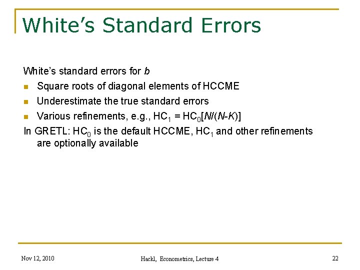
White’s Standard Errors White’s standard errors for b n Square roots of diagonal elements of HCCME Underestimate the true standard errors n Various refinements, e. g. , HC 1 = HC 0[N/(N-K)] In GRETL: HC 0 is the default HCCME, HC 1 and other refinements are optionally available n Nov 12, 2010 Hackl, Econometrics, Lecture 4 22

An Alternative Estimator for b Idea of the estimator n Transform the model so that it satisfies the Gauss-Markov assumptions n Apply OLS to the transformed model n Results in a BLUE Transformation often depends upon unknown parameters that characterizing heteroskedasticity: two-step procedure 1. Estimate the parameters that characterize heteroskedasticity and transform the model 2. Estimate the transformed model The procedure results in an approximately BLUE Nov 12, 2010 Hackl, Econometrics, Lecture 4 23

An Example Model: yi = xi’β + εi with V{εi} = σi 2 = σ2 hi 2 Division by hi results in yi /hi = (xi /hi)’β + εi /hi with a homoskedastic error term V{εi /hi} = σi 2/hi 2 = σ2 OLS applied to the transformed model gives It is called a generalized least squares (GLS) or weighted least squares (WLS) estimator Nov 12, 2010 Hackl, Econometrics, Lecture 4 24

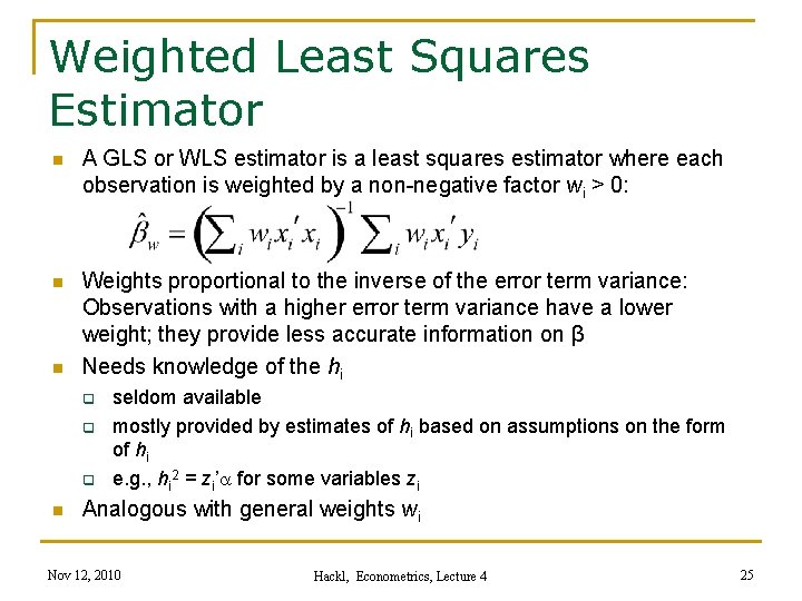
Weighted Least Squares Estimator n A GLS or WLS estimator is a least squares estimator where each observation is weighted by a non-negative factor wi > 0: n Weights proportional to the inverse of the error term variance: Observations with a higher error term variance have a lower weight; they provide less accurate information on β Needs knowledge of the hi n q q q n seldom available mostly provided by estimates of hi based on assumptions on the form of hi e. g. , hi 2 = zi’a for some variables zi Analogous with general weights wi Nov 12, 2010 Hackl, Econometrics, Lecture 4 25

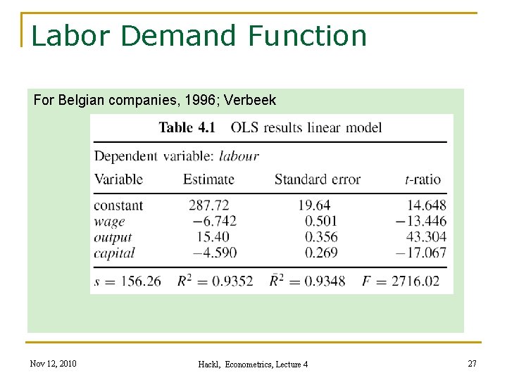
Example: Labor Demand Verbeek’s data set “labour 2”: Sample of 569 Belgian companies (data from 1996) n n Variables q labour: total employment (number of employees) q capital: total fixed assets q wage: total wage costs per employee (in 1000 EUR) q output: value added (in million EUR) Labour demand function labour = b 1 + b 2*wage + b 3*output + b 4*capital Nov 12, 2010 Hackl, Econometrics, Lecture 4 26

Labor Demand Function For Belgian companies, 1996; Verbeek Nov 12, 2010 Hackl, Econometrics, Lecture 4 27

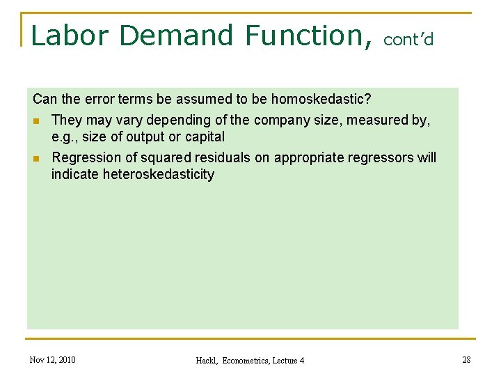
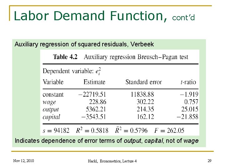
Labor Demand Function, cont’d Can the error terms be assumed to be homoskedastic? n They may vary depending of the company size, measured by, e. g. , size of output or capital n Regression of squared residuals on appropriate regressors will indicate heteroskedasticity Nov 12, 2010 Hackl, Econometrics, Lecture 4 28

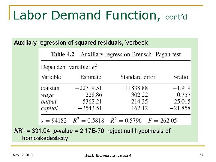
Labor Demand Function, cont’d Auxiliary regression of squared residuals, Verbeek Indicates dependence of error terms of output, capital, not of wage Nov 12, 2010 Hackl, Econometrics, Lecture 4 29

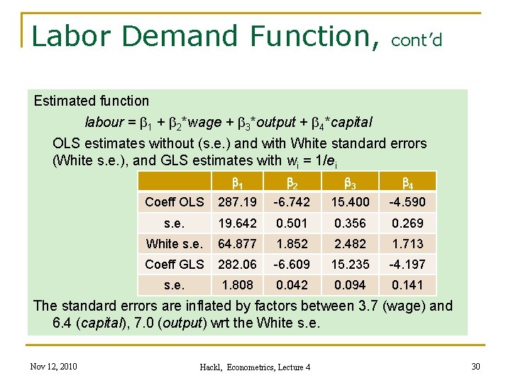
Labor Demand Function, cont’d Estimated function labour = b 1 + b 2*wage + b 3*output + b 4*capital OLS estimates without (s. e. ) and with White standard errors (White s. e. ), and GLS estimates with wi = 1/ei b 1 b 2 b 3 b 4 Coeff OLS 287. 19 -6. 742 15. 400 -4. 590 s. e. 19. 642 0. 501 0. 356 0. 269 White s. e. 64. 877 1. 852 2. 482 1. 713 Coeff GLS 282. 06 -6. 609 15. 235 -4. 197 s. e. 1. 808 0. 042 0. 094 0. 141 The standard errors are inflated by factors between 3. 7 (wage) and 6. 4 (capital), 7. 0 (output) wrt the White s. e. Nov 12, 2010 Hackl, Econometrics, Lecture 4 30

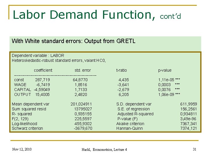
Labor Demand Function, cont’d With White standard errors: Output from GRETL Dependent variable : LABOR Heteroskedastic-robust standard errors, vaiant HC 0, coefficient std. error ------------------------------const 287, 719 64, 8770 WAGE -6, 7419 1, 8516 CAPITAL -4, 59049 1, 7133 OUTPUT 15, 4005 2, 4820 Mean dependent var Sum squared resid R- squared F(2, 129) Log-likelihood Schwarz criterion Nov 12, 2010 201, 024911 13795027 0, 935155 225, 5597 455, 9302 -3679, 670 t-ratio p-value 4, 435 -3, 641 -2, 679 6, 205 1, 11 e-05 *** 0, 0003 *** 0, 0076 *** 1, 06 e-09 *** S. D. dependent var S. E. of regression Adjusted R-squared P-value (F) Akaike criterion Hannan-Quinn Hackl, Econometrics, Lecture 4 611, 9959 156, 2561 0, 934811 3, 49 e-96 7367, 341 7374, 121 31

Tests against Heteroskedasticity Due to unbiasedness of b, residuals are expected to indicate heteroskedasticity Graphical displays of residuals may give useful hints Residual-based tests: n Breusch-Pagan test n Goldfeld-Quandt test n White test Nov 12, 2010 Hackl, Econometrics, Lecture 4 32

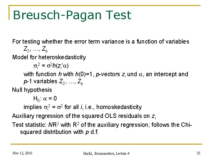
Breusch-Pagan Test For testing whether the error term variance is a function of variables Z 2, …, Zp Model for heteroskedasticity si 2 = s 2 h(zi‘a) with function h with h(0)=1, p-vectors zi und a, an intercept and p-1 variables Z 2, …, Zp Null hypothesis H 0 : a = 0 implies si 2 = s 2 for all i, i. e. , homoskedasticity Auxiliary regression of the squared OLS residuals on zi Test statistic: NR 2 with R 2 of the auxiliary regression; follows the Chisquared distribution with p d. f. Nov 12, 2010 Hackl, Econometrics, Lecture 4 33

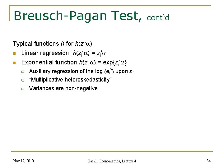
Breusch-Pagan Test, cont‘d Typical functions h for h(zi‘a) n Linear regression: h(zi‘a) = zi‘a n Exponential function h(zi‘a) = exp{zi‘a} q Auxiliary regression of the log (ei 2) upon zi q “Multiplicative heteroskedasticity” q Variances are non-negative Nov 12, 2010 Hackl, Econometrics, Lecture 4 34

Labor Demand Function, cont’d Auxiliary regression of squared residuals, Verbeek NR 2 = 331. 04, p-value = 2. 17 E-70; reject null hypothesis of homoskedasticity Nov 12, 2010 Hackl, Econometrics, Lecture 4 35

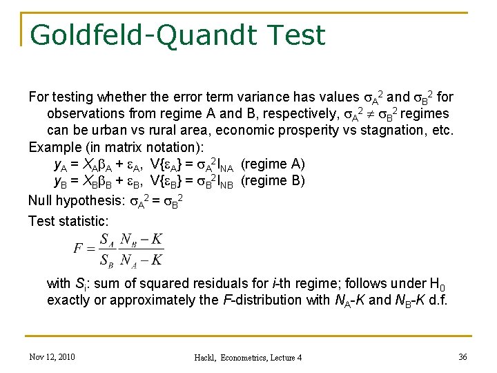
Goldfeld-Quandt Test For testing whether the error term variance has values s. A 2 and s. B 2 for observations from regime A and B, respectively, s. A 2 s. B 2 regimes can be urban vs rural area, economic prosperity vs stagnation, etc. Example (in matrix notation): y. A = XAb. A + e. A, V{e. A} = s. A 2 INA (regime A) y. B = XBb. B + e. B, V{e. B} = s. B 2 INB (regime B) Null hypothesis: s. A 2 = s. B 2 Test statistic: with Si: sum of squared residuals for i-th regime; follows under H 0 exactly or approximately the F-distribution with NA-K and NB-K d. f. Nov 12, 2010 Hackl, Econometrics, Lecture 4 36

Goldfeld-Quandt Test, cont‘d Test procedure in three steps: 1. Sort the observations with respect to the regimes 2. Separate fittings of the model to the NA and NB observations; sum of squared residuals SA and SB 3. Calculation of test statistic F Nov 12, 2010 Hackl, Econometrics, Lecture 4 37

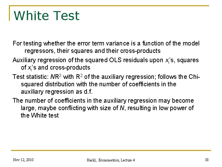
White Test For testing whether the error term variance is a function of the model regressors, their squares and their cross-products Auxiliary regression of the squared OLS residuals upon xi’s, squares of xi’s and cross-products Test statistic: NR 2 with R 2 of the auxiliary regression; follows the Chisquared distribution with the number of coefficients in the auxiliary regression as d. f. The number of coefficients in the auxiliary regression may become large, maybe conflicting with size of N, resulting in low power of the White test Nov 12, 2010 Hackl, Econometrics, Lecture 4 38

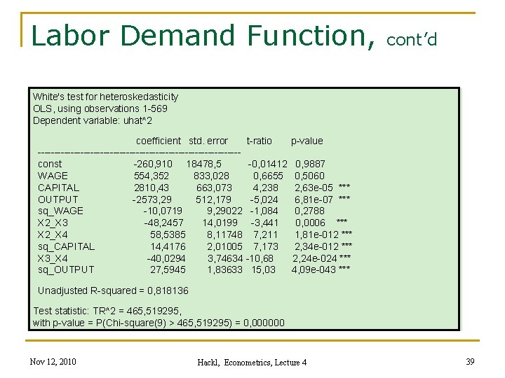
Labor Demand Function, cont’d White's test for heteroskedasticity OLS, using observations 1 -569 Dependent variable: uhat^2 coefficient std. error t-ratio -------------------------------const -260, 910 18478, 5 -0, 01412 WAGE 554, 352 833, 028 0, 6655 CAPITAL 2810, 43 663, 073 4, 238 OUTPUT -2573, 29 512, 179 -5, 024 sq_WAGE -10, 0719 9, 29022 -1, 084 X 2_X 3 -48, 2457 14, 0199 -3, 441 X 2_X 4 58, 5385 8, 11748 7, 211 sq_CAPITAL 14, 4176 2, 01005 7, 173 X 3_X 4 -40, 0294 3, 74634 -10, 68 sq_OUTPUT 27, 5945 1, 83633 15, 03 p-value 0, 9887 0, 5060 2, 63 e-05 *** 6, 81 e-07 *** 0, 2788 0, 0006 *** 1, 81 e-012 *** 2, 34 e-012 *** 2, 24 e-024 *** 4, 09 e-043 *** Unadjusted R-squared = 0, 818136 Test statistic: TR^2 = 465, 519295, with p-value = P(Chi-square(9) > 465, 519295) = 0, 000000 Nov 12, 2010 Hackl, Econometrics, Lecture 4 39

Contents n n Violations of V{ε} = s 2 IN Heteroskedasticity GLS Estimation Autocorrelation Nov 12, 2010 Hackl, Econometrics, Lecture 4 40

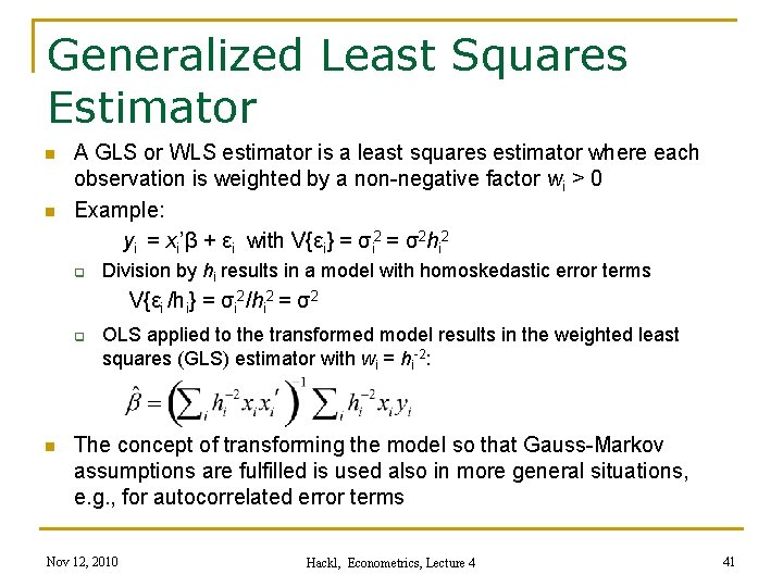
Generalized Least Squares Estimator n n A GLS or WLS estimator is a least squares estimator where each observation is weighted by a non-negative factor wi > 0 Example: yi = xi’β + εi with V{εi} = σi 2 = σ2 hi 2 q Division by hi results in a model with homoskedastic error terms V{εi /hi} = σi 2/hi 2 = σ2 q n OLS applied to the transformed model results in the weighted least squares (GLS) estimator with wi = hi-2: The concept of transforming the model so that Gauss-Markov assumptions are fulfilled is used also in more general situations, e. g. , for autocorrelated error terms Nov 12, 2010 Hackl, Econometrics, Lecture 4 41

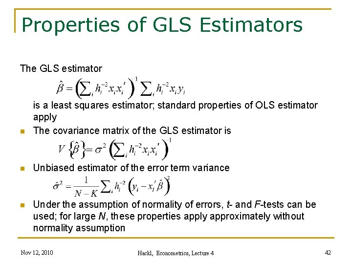
Properties of GLS Estimators The GLS estimator n is a least squares estimator; standard properties of OLS estimator apply The covariance matrix of the GLS estimator is n Unbiased estimator of the error term variance n Under the assumption of normality of errors, t- and F-tests can be used; for large N, these properties apply approximately without normality assumption Nov 12, 2010 Hackl, Econometrics, Lecture 4 42

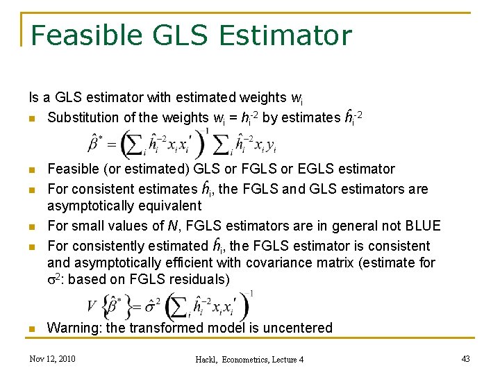
Feasible GLS Estimator Is a GLS estimator with estimated weights wi n Substitution of the weights wi = hi-2 by estimates ĥi-2 n n n Feasible (or estimated) GLS or FGLS or EGLS estimator For consistent estimates ĥi, the FGLS and GLS estimators are asymptotically equivalent For small values of N, FGLS estimators are in general not BLUE For consistently estimated ĥi, the FGLS estimator is consistent and asymptotically efficient with covariance matrix (estimate for s 2: based on FGLS residuals) Warning: the transformed model is uncentered Nov 12, 2010 Hackl, Econometrics, Lecture 4 43

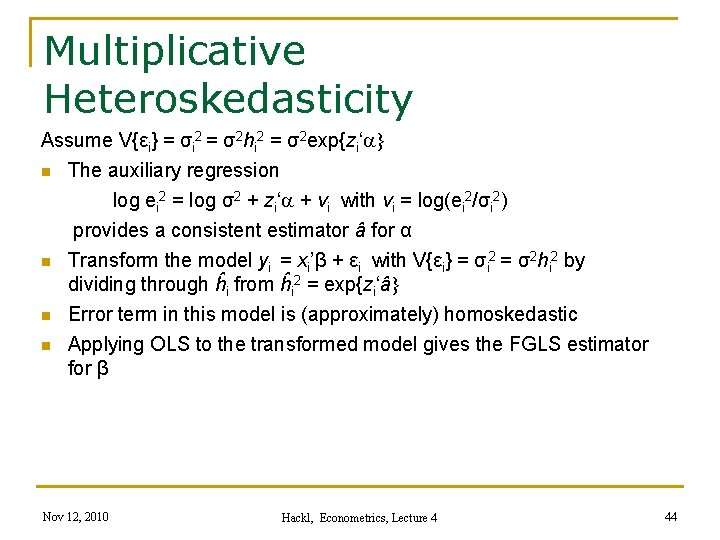
Multiplicative Heteroskedasticity Assume V{εi} = σi 2 = σ2 hi 2 = σ2 exp{zi‘a} n The auxiliary regression n log ei 2 = log σ2 + zi‘a + vi with vi = log(ei 2/σi 2) provides a consistent estimator â for α Transform the model yi = xi’β + εi with V{εi} = σi 2 = σ2 hi 2 by dividing through ĥi from ĥi 2 = exp{zi‘â} Error term in this model is (approximately) homoskedastic Applying OLS to the transformed model gives the FGLS estimator for β Nov 12, 2010 Hackl, Econometrics, Lecture 4 44

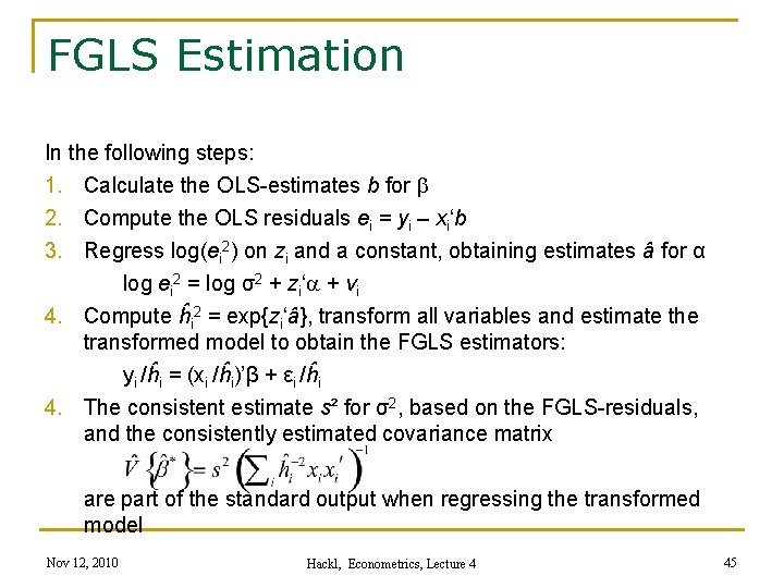
FGLS Estimation In the following steps: 1. Calculate the OLS-estimates b for b 2. Compute the OLS residuals ei = yi – xi‘b 3. Regress log(ei 2) on zi and a constant, obtaining estimates â for α log ei 2 = log σ2 + zi‘a + vi 4. Compute ĥi 2 = exp{zi‘â}, transform all variables and estimate the transformed model to obtain the FGLS estimators: yi /ĥi = (xi /ĥi)’β + εi /ĥi 4. The consistent estimate s² for σ2, based on the FGLS-residuals, and the consistently estimated covariance matrix are part of the standard output when regressing the transformed model Nov 12, 2010 Hackl, Econometrics, Lecture 4 45

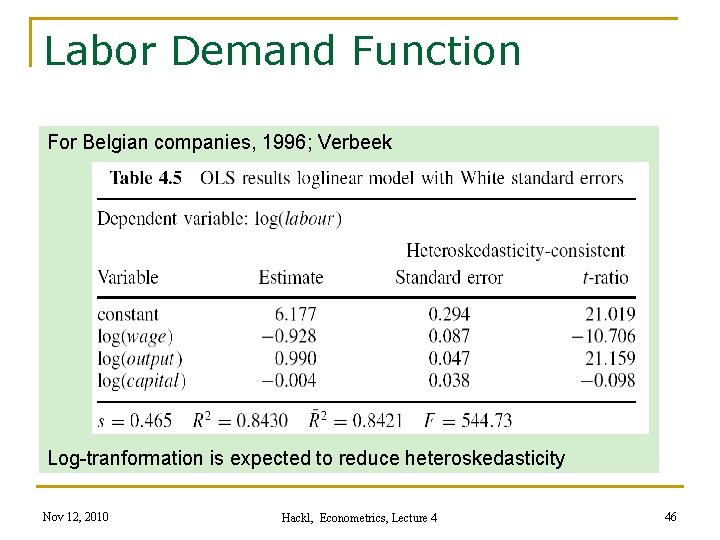
Labor Demand Function For Belgian companies, 1996; Verbeek Log-tranformation is expected to reduce heteroskedasticity Nov 12, 2010 Hackl, Econometrics, Lecture 4 46

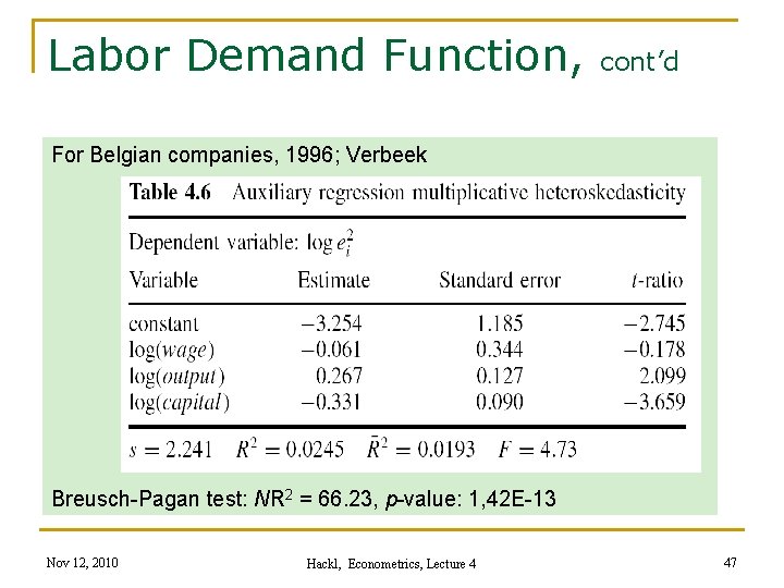
Labor Demand Function, cont’d For Belgian companies, 1996; Verbeek Breusch-Pagan test: NR 2 = 66. 23, p-value: 1, 42 E-13 Nov 12, 2010 Hackl, Econometrics, Lecture 4 47

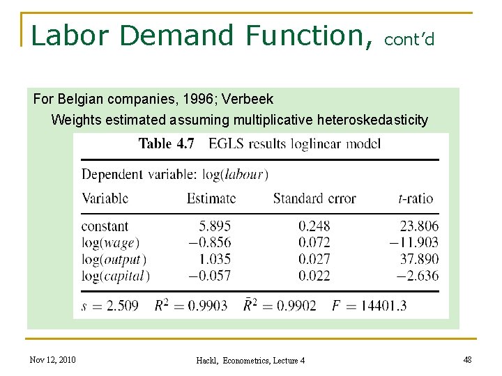
Labor Demand Function, cont’d For Belgian companies, 1996; Verbeek Weights estimated assuming multiplicative heteroskedasticity Nov 12, 2010 Hackl, Econometrics, Lecture 4 48

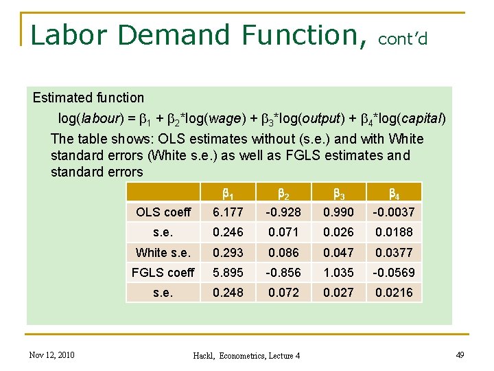
Labor Demand Function, cont’d Estimated function log(labour) = b 1 + b 2*log(wage) + b 3*log(output) + b 4*log(capital) The table shows: OLS estimates without (s. e. ) and with White standard errors (White s. e. ) as well as FGLS estimates and standard errors Nov 12, 2010 b 1 b 2 b 3 b 4 OLS coeff 6. 177 -0. 928 0. 990 -0. 0037 s. e. 0. 246 0. 071 0. 026 0. 0188 White s. e. 0. 293 0. 086 0. 047 0. 0377 FGLS coeff 5. 895 -0. 856 1. 035 -0. 0569 s. e. 0. 248 0. 072 0. 027 0. 0216 Hackl, Econometrics, Lecture 4 49

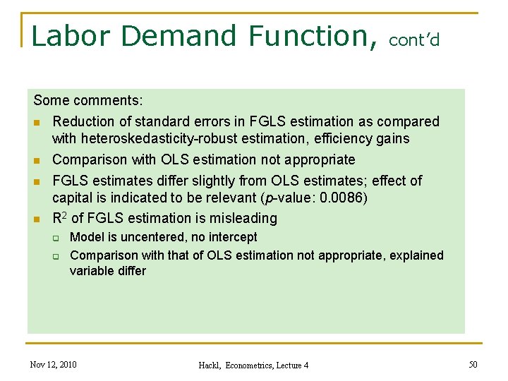
Labor Demand Function, cont’d Some comments: n Reduction of standard errors in FGLS estimation as compared with heteroskedasticity-robust estimation, efficiency gains n Comparison with OLS estimation not appropriate n FGLS estimates differ slightly from OLS estimates; effect of capital is indicated to be relevant (p-value: 0. 0086) n R 2 of FGLS estimation is misleading q q Model is uncentered, no intercept Comparison with that of OLS estimation not appropriate, explained variable differ Nov 12, 2010 Hackl, Econometrics, Lecture 4 50

Contents n n Violations of V{ε} = s 2 IN Heteroskedasticity GLS Estimation Autocorrelation Nov 12, 2010 Hackl, Econometrics, Lecture 4 51

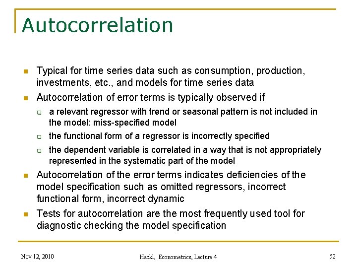
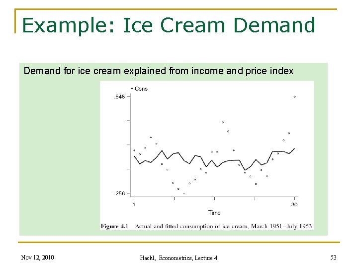
Autocorrelation n Typical for time series data such as consumption, production, investments, etc. , and models for time series data n Autocorrelation of error terms is typically observed if q q q n n a relevant regressor with trend or seasonal pattern is not included in the model: miss-specified model the functional form of a regressor is incorrectly specified the dependent variable is correlated in a way that is not appropriately represented in the systematic part of the model Autocorrelation of the error terms indicates deficiencies of the model specification such as omitted regressors, incorrect functional form, incorrect dynamic Tests for autocorrelation are the most frequently used tool for diagnostic checking the model specification Nov 12, 2010 Hackl, Econometrics, Lecture 4 52

Example: Ice Cream Demand for ice cream explained from income and price index Nov 12, 2010 Hackl, Econometrics, Lecture 4 53

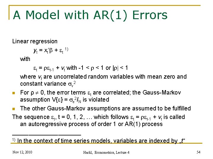
A Model with AR(1) Errors Linear regression yt = xt‘b + et 1) with et = ret-1 + vt with -1 < r < 1 or |r| < 1 where vt are uncorrelated random variables with mean zero and constant variance sv 2 n For ρ 0, the error terms et are correlated; the Gauss-Markov assumption V{e} = se 2 IN is violated n The other Gauss-Markov assumptions are assumed to be fulfilled The sequence et, t = 0, 1, 2, … which follows et = ret-1 + vt is called an autoregressive process of order 1 or AR(1) process ___________ 1) In the context of time series models, variables are indexed by „t“ Nov 12, 2010 Hackl, Econometrics, Lecture 4 54

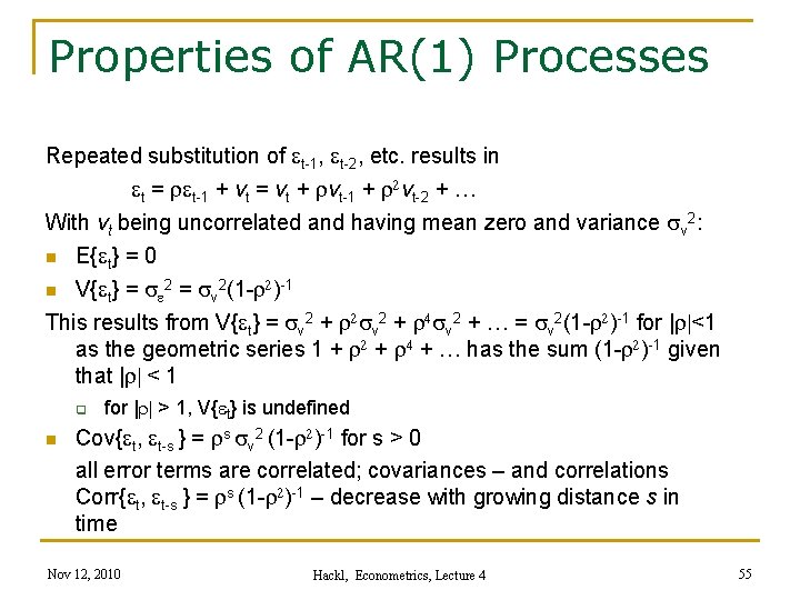
Properties of AR(1) Processes Repeated substitution of et-1, et-2, etc. results in et = ret-1 + vt = vt + rvt-1 + r 2 vt-2 + … With vt being uncorrelated and having mean zero and variance sv 2: n E{et} = 0 n V{et} = se 2 = sv 2(1 -r 2)-1 This results from V{et} = sv 2 + r 2 sv 2 + r 4 sv 2 + … = sv 2(1 -r 2)-1 for |r|<1 as the geometric series 1 + r 2 + r 4 + … has the sum (1 -r 2)-1 given that |r| < 1 q n for |r| > 1, V{et} is undefined Cov{et, et-s } = rs sv 2 (1 -r 2)-1 for s > 0 all error terms are correlated; covariances – and correlations Corr{et, et-s } = rs (1 -r 2)-1 – decrease with growing distance s in time Nov 12, 2010 Hackl, Econometrics, Lecture 4 55

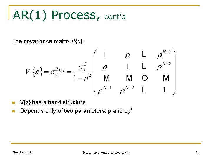
AR(1) Process, cont’d The covariance matrix V{e}: n n V{e} has a band structure Depends only of two parameters: r and sv 2 Nov 12, 2010 Hackl, Econometrics, Lecture 4 56

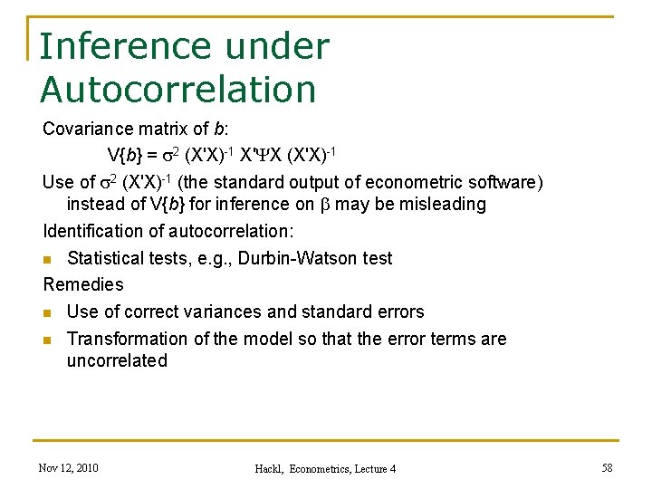
Consequences of V{e} s 2 IT OLS-estimators b for b n are unbiased are consistent n have the covariance-matrix V{b} = s 2 (X'X)-1 X'YX (X'X)-1 n are not efficient estimators, not BLUE n follow – under general conditions – asymptotically the normal distribution The estimator s 2 = e'e/(T-K) for s 2 is biased For an AR(1)-process et with r > 0, s. e. from s 2 (X'X)-1 underestimates the true s. e. n Nov 12, 2010 Hackl, Econometrics, Lecture 4 57

Inference under Autocorrelation Covariance matrix of b: V{b} = s 2 (X'X)-1 X'YX (X'X)-1 Use of s 2 (X'X)-1 (the standard output of econometric software) instead of V{b} for inference on b may be misleading Identification of autocorrelation: n Statistical tests, e. g. , Durbin-Watson test Remedies n Use of correct variances and standard errors n Transformation of the model so that the error terms are uncorrelated Nov 12, 2010 Hackl, Econometrics, Lecture 4 58

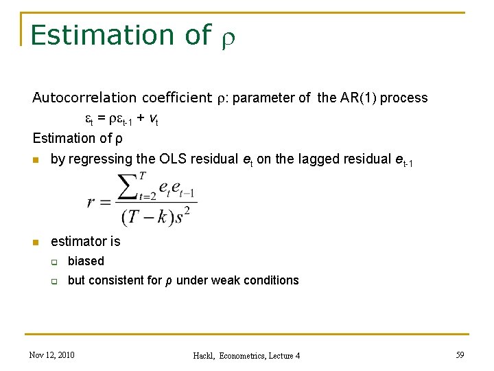
Estimation of r Autocorrelation coefficient r: parameter of the AR(1) process et = ret-1 + vt Estimation of ρ n by regressing the OLS residual et on the lagged residual et-1 n estimator is q biased q but consistent for ρ under weak conditions Nov 12, 2010 Hackl, Econometrics, Lecture 4 59

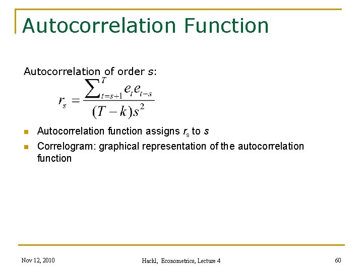
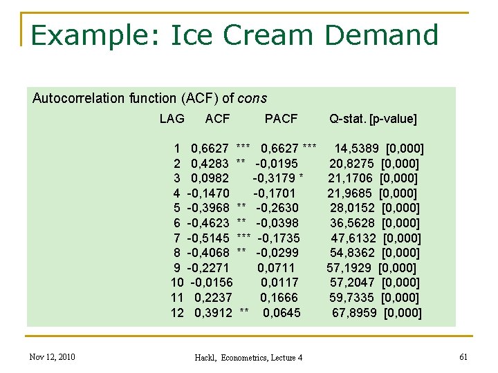
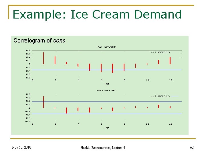
Autocorrelation Function Autocorrelation of order s: n n Autocorrelation function assigns rs to s Correlogram: graphical representation of the autocorrelation function Nov 12, 2010 Hackl, Econometrics, Lecture 4 60

Example: Ice Cream Demand Autocorrelation function (ACF) of cons LAG ACF PACF 1 0, 6627 *** 2 0, 4283 ** -0, 0195 3 0, 0982 -0, 3179 * 4 -0, 1470 -0, 1701 5 -0, 3968 ** -0, 2630 6 -0, 4623 ** -0, 0398 7 -0, 5145 *** -0, 1735 8 -0, 4068 ** -0, 0299 9 -0, 2271 0, 0711 10 -0, 0156 0, 0117 11 0, 2237 0, 1666 12 0, 3912 ** 0, 0645 Nov 12, 2010 Hackl, Econometrics, Lecture 4 Q-stat. [p-value] 14, 5389 [0, 000] 20, 8275 [0, 000] 21, 1706 [0, 000] 21, 9685 [0, 000] 28, 0152 [0, 000] 36, 5628 [0, 000] 47, 6132 [0, 000] 54, 8362 [0, 000] 57, 1929 [0, 000] 57, 2047 [0, 000] 59, 7335 [0, 000] 67, 8959 [0, 000] 61

Example: Ice Cream Demand Correlogram of cons Nov 12, 2010 Hackl, Econometrics, Lecture 4 62

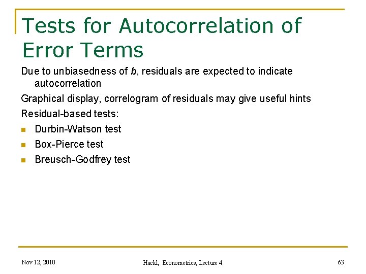
Tests for Autocorrelation of Error Terms Due to unbiasedness of b, residuals are expected to indicate autocorrelation Graphical display, correlogram of residuals may give useful hints Residual-based tests: n Durbin-Watson test n Box-Pierce test n Breusch-Godfrey test Nov 12, 2010 Hackl, Econometrics, Lecture 4 63

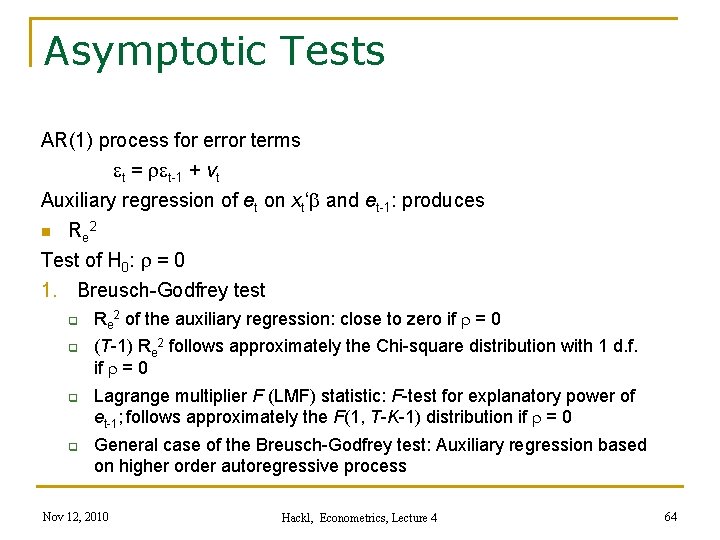
Asymptotic Tests AR(1) process for error terms et = ret-1 + vt Auxiliary regression of et on xt‘b and et-1: produces n Re 2 Test of H 0: r = 0 1. Breusch-Godfrey test q q Re 2 of the auxiliary regression: close to zero if r = 0 (T-1) Re 2 follows approximately the Chi-square distribution with 1 d. f. if r = 0 Lagrange multiplier F (LMF) statistic: F-test for explanatory power of et-1; follows approximately the F(1, T-K-1) distribution if r = 0 General case of the Breusch-Godfrey test: Auxiliary regression based on higher order autoregressive process Nov 12, 2010 Hackl, Econometrics, Lecture 4 64

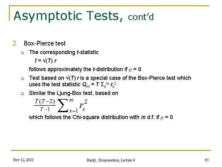
Asymptotic Tests, cont’d 2. Box-Pierce test q The corresponding t-statistic t = √(T) r follows approximately the t-distribution if r = 0 q q Test based on √(T) r is a special case of the Box-Pierce test which uses the test statistic Qm = T Σsm rs 2 Similar the Ljung-Box test, based on which follows the Chi-square distribution with m d. f. if r = 0 Nov 12, 2010 Hackl, Econometrics, Lecture 4 65

Asymptotic Tests, cont’d Remarks n If the model of interest contains lagged values of y the auxiliary regression should also include all explanatory variables (just to make sure the distribution of the test is correct) n If heteroskedasticity is suspected, White standard errors may be used in the auxiliary regression Nov 12, 2010 Hackl, Econometrics, Lecture 4 66

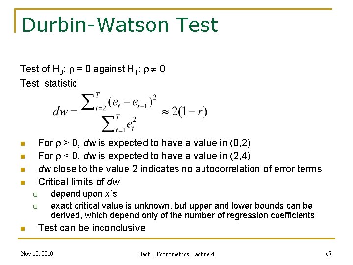
Durbin-Watson Test of H 0: r = 0 against H 1: r 0 Test statistic For r > 0, dw is expected to have a value in (0, 2) For r < 0, dw is expected to have a value in (2, 4) dw close to the value 2 indicates no autocorrelation of error terms Critical limits of dw n n q q n depend upon xt’s exact critical value is unknown, but upper and lower bounds can be derived, which depend only of the number of regression coefficients Test can be inconclusive Nov 12, 2010 Hackl, Econometrics, Lecture 4 67

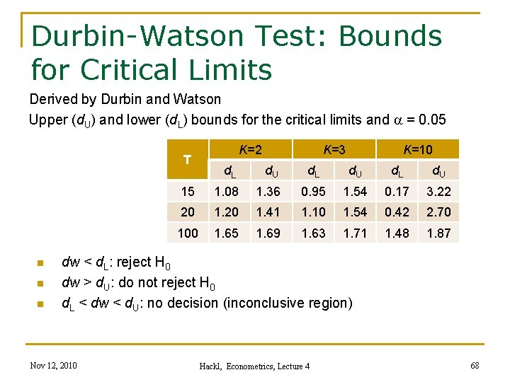
Durbin-Watson Test: Bounds for Critical Limits Derived by Durbin and Watson Upper (d. U) and lower (d. L) bounds for the critical limits and a = 0. 05 T n n n K=2 K=3 K=10 d. L d. U 15 1. 08 1. 36 0. 95 1. 54 0. 17 3. 22 20 1. 41 1. 10 1. 54 0. 42 2. 70 100 1. 65 1. 69 1. 63 1. 71 1. 48 1. 87 dw < d. L: reject H 0 dw > d. U: do not reject H 0 d. L < dw < d. U: no decision (inconclusive region) Nov 12, 2010 Hackl, Econometrics, Lecture 4 68

Durbin-Watson Test: Remarks Durbin-Watson test gives no reference to causes of rejection of the null hypothesis and how the model to modify Causes for rejection of the null hypothesis can be various types of misspecification Durbin-Watson test is a test against first-order autocorrelation; a test against autocorrelation of other orders may be more suitable, e. g. , order four if the model is for quarterly data Use of tables unwieldy n n q q Limited number of critical bounds (K, T, a) in tables Inconclusive region Nov 12, 2010 Hackl, Econometrics, Lecture 4 69

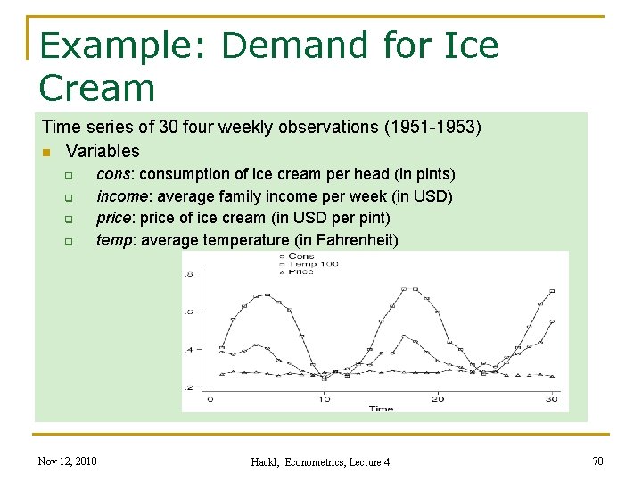
Example: Demand for Ice Cream Time series of 30 four weekly observations (1951 -1953) n Variables q q cons: consumption of ice cream per head (in pints) income: average family income per week (in USD) price: price of ice cream (in USD per pint) temp: average temperature (in Fahrenheit) Nov 12, 2010 Hackl, Econometrics, Lecture 4 70

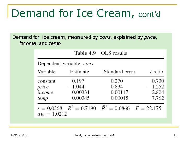
Demand for Ice Cream, cont’d Demand for ice cream, measured by cons, explained by price, income, and temp Nov 12, 2010 Hackl, Econometrics, Lecture 4 71

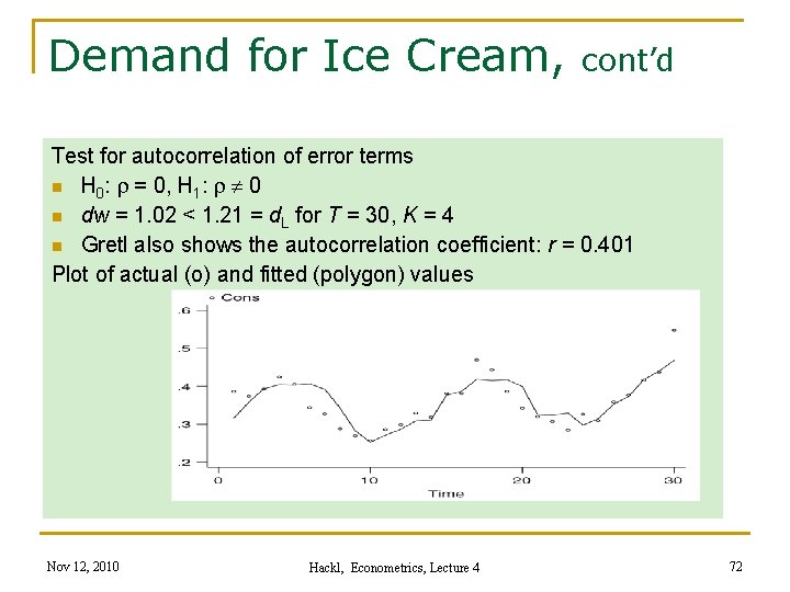
Demand for Ice Cream, cont’d Test for autocorrelation of error terms n H 0: r = 0, H 1: r 0 n dw = 1. 02 < 1. 21 = d. L for T = 30, K = 4 n Gretl also shows the autocorrelation coefficient: r = 0. 401 Plot of actual (o) and fitted (polygon) values Nov 12, 2010 Hackl, Econometrics, Lecture 4 72

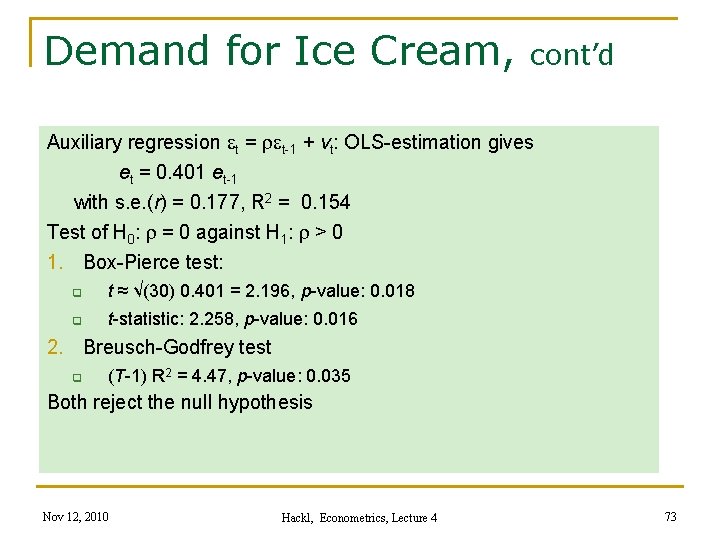
Demand for Ice Cream, cont’d Auxiliary regression et = ret-1 + vt: OLS-estimation gives et = 0. 401 et-1 with s. e. (r) = 0. 177, R 2 = 0. 154 Test of H 0: r = 0 against H 1: r > 0 1. Box-Pierce test: q t ≈ √(30) 0. 401 = 2. 196, p-value: 0. 018 q t-statistic: 2. 258, p-value: 0. 016 2. Breusch-Godfrey test q (T-1) R 2 = 4. 47, p-value: 0. 035 Both reject the null hypothesis Nov 12, 2010 Hackl, Econometrics, Lecture 4 73

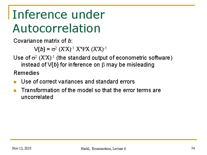
Inference under Autocorrelation Covariance matrix of b: V{b} = s 2 (X'X)-1 X'YX (X'X)-1 Use of s 2 (X'X)-1 (the standard output of econometric software) instead of V{b} for inference on b may be misleading Remedies n Use of correct variances and standard errors n Transformation of the model so that the error terms are uncorrelated Nov 12, 2010 Hackl, Econometrics, Lecture 4 74

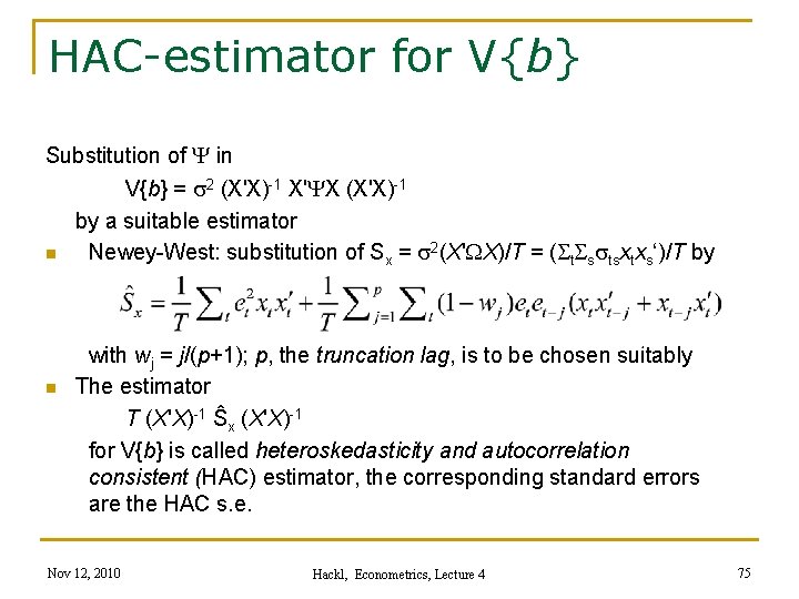
HAC-estimator for V{b} Substitution of Y in V{b} = s 2 (X'X)-1 X'YX (X'X)-1 by a suitable estimator n Newey-West: substitution of Sx = s 2(X'WX)/T = (St. Ssstsxtxs‘)/T by n with wj = j/(p+1); p, the truncation lag, is to be chosen suitably The estimator T (X'X)-1 Ŝx (X'X)-1 for V{b} is called heteroskedasticity and autocorrelation consistent (HAC) estimator, the corresponding standard errors are the HAC s. e. Nov 12, 2010 Hackl, Econometrics, Lecture 4 75

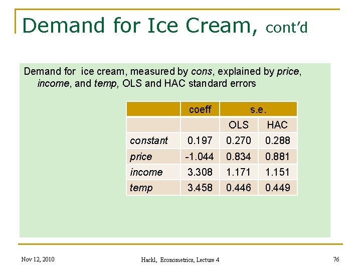
Demand for Ice Cream, cont’d Demand for ice cream, measured by cons, explained by price, income, and temp, OLS and HAC standard errors coeff Nov 12, 2010 s. e. OLS HAC constant 0. 197 0. 270 0. 288 price -1. 044 0. 834 0. 881 income 3. 308 1. 171 1. 151 temp 3. 458 0. 446 0. 449 Hackl, Econometrics, Lecture 4 76

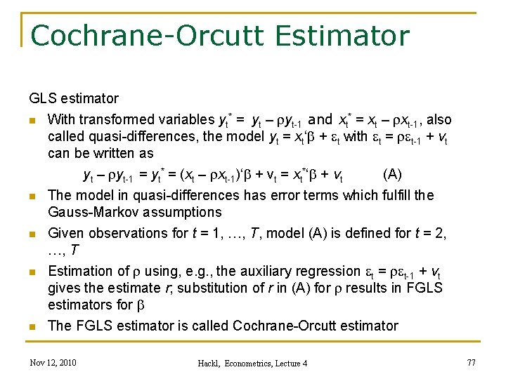
Cochrane-Orcutt Estimator GLS estimator n With transformed variables yt* = yt – ryt-1 and xt* = xt – rxt-1, also called quasi-differences, the model yt = xt‘b + et with et = ret-1 + vt can be written as yt – ryt-1 = yt* = (xt – rxt-1)‘b + vt = xt*‘b + vt (A) n The model in quasi-differences has error terms which fulfill the Gauss-Markov assumptions n Given observations for t = 1, …, T, model (A) is defined for t = 2, …, T n Estimation of r using, e. g. , the auxiliary regression et = ret-1 + vt gives the estimate r; substitution of r in (A) for r results in FGLS estimators for b n The FGLS estimator is called Cochrane-Orcutt estimator Nov 12, 2010 Hackl, Econometrics, Lecture 4 77

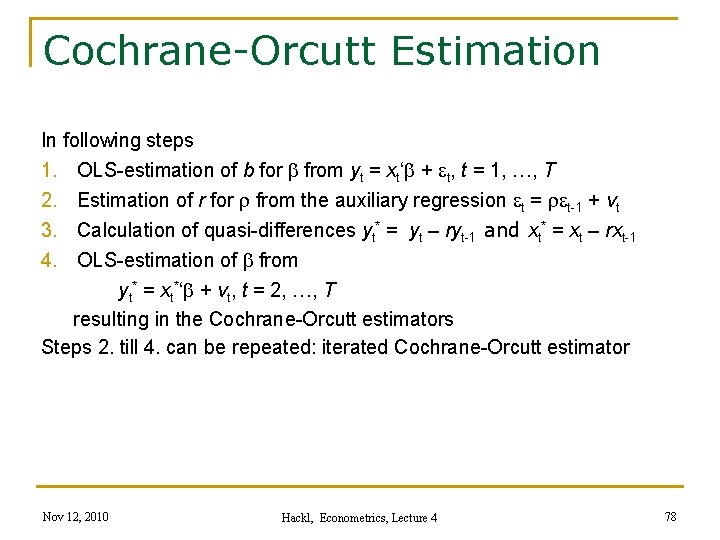
Cochrane-Orcutt Estimation In following steps 1. OLS-estimation of b for b from yt = xt‘b + et, t = 1, …, T 2. Estimation of r for r from the auxiliary regression et = ret-1 + vt 3. Calculation of quasi-differences yt* = yt – ryt-1 and xt* = xt – rxt-1 4. OLS-estimation of b from yt* = xt*‘b + vt, t = 2, …, T resulting in the Cochrane-Orcutt estimators Steps 2. till 4. can be repeated: iterated Cochrane-Orcutt estimator Nov 12, 2010 Hackl, Econometrics, Lecture 4 78

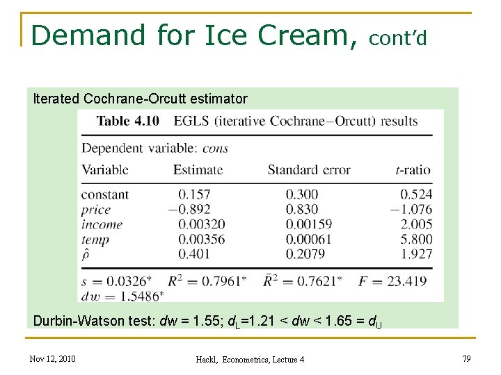
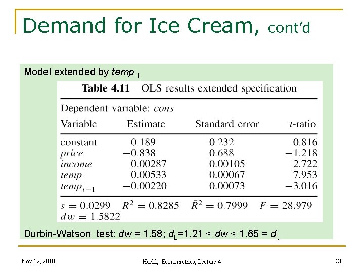
Demand for Ice Cream, cont’d Iterated Cochrane-Orcutt estimator Durbin-Watson test: dw = 1. 55; d. L=1. 21 < dw < 1. 65 = d. U Nov 12, 2010 Hackl, Econometrics, Lecture 4 79

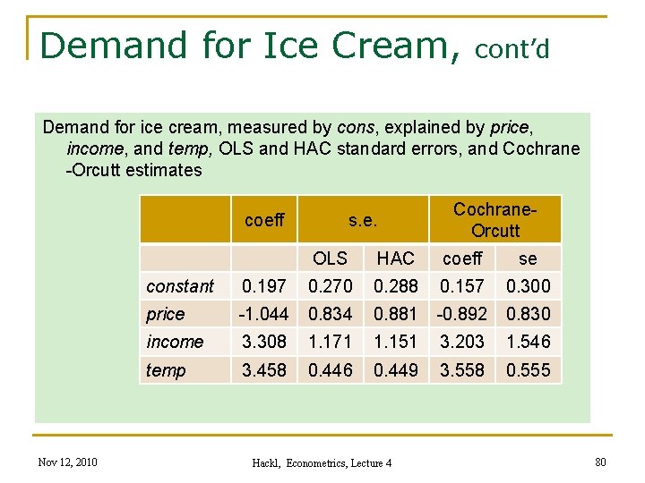
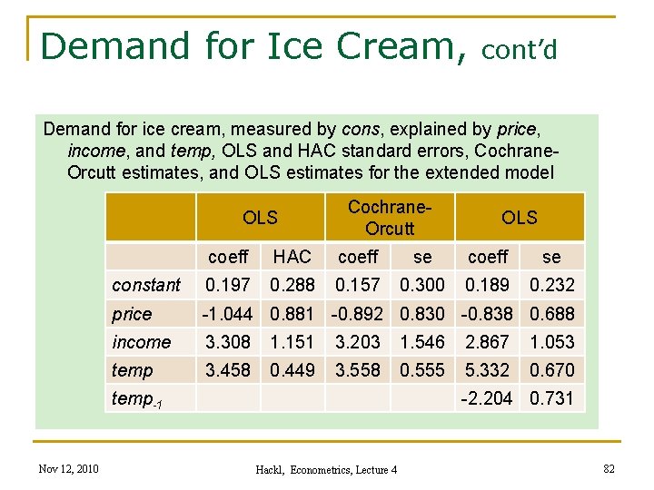
Demand for Ice Cream, cont’d Demand for ice cream, measured by cons, explained by price, income, and temp, OLS and HAC standard errors, and Cochrane -Orcutt estimates coeff Nov 12, 2010 s. e. Cochrane. Orcutt OLS HAC coeff se constant 0. 197 0. 270 0. 288 0. 157 0. 300 price -1. 044 0. 834 0. 881 -0. 892 0. 830 income 3. 308 1. 171 1. 151 3. 203 1. 546 temp 3. 458 0. 446 0. 449 3. 558 0. 555 Hackl, Econometrics, Lecture 4 80

Demand for Ice Cream, cont’d Model extended by temp-1 Durbin-Watson test: dw = 1. 58; d. L=1. 21 < dw < 1. 65 = d. U Nov 12, 2010 Hackl, Econometrics, Lecture 4 81

Demand for Ice Cream, cont’d Demand for ice cream, measured by cons, explained by price, income, and temp, OLS and HAC standard errors, Cochrane. Orcutt estimates, and OLS estimates for the extended model OLS Cochrane. Orcutt coeff HAC coeff se constant 0. 197 0. 288 0. 157 0. 300 0. 189 0. 232 price -1. 044 0. 881 -0. 892 0. 830 -0. 838 0. 688 income 3. 308 1. 151 3. 203 1. 546 2. 867 1. 053 temp 3. 458 0. 449 3. 558 0. 555 5. 332 0. 670 temp-1 Nov 12, 2010 OLS -2. 204 0. 731 Hackl, Econometrics, Lecture 4 82

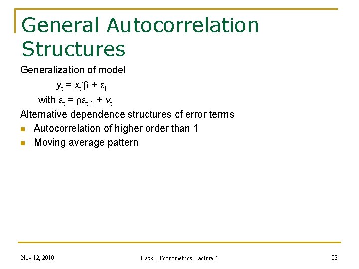
General Autocorrelation Structures Generalization of model yt = xt‘b + et with et = ret-1 + vt Alternative dependence structures of error terms n Autocorrelation of higher order than 1 n Moving average pattern Nov 12, 2010 Hackl, Econometrics, Lecture 4 83

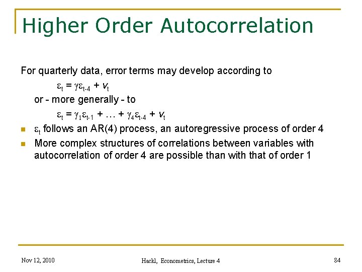
Higher Order Autocorrelation For quarterly data, error terms may develop according to et = get-4 + vt or - more generally - to et = g 1 et-1 + … + g 4 et-4 + vt n et follows an AR(4) process, an autoregressive process of order 4 n More complex structures of correlations between variables with autocorrelation of order 4 are possible than with that of order 1 Nov 12, 2010 Hackl, Econometrics, Lecture 4 84

Moving Average Processes Moving average process of order 1, MA(1) process et = vt + avt-1 n n εt is correlated with εt-1, but not with εt-2, εt-3, … Generalizations to higher orders Nov 12, 2010 Hackl, Econometrics, Lecture 4 85

Remedies against Autocorrelation n n Change functional form, e. g. , use log(y) instead of y Extend the model by including additional explanatory variables, e. g. , seasonal dummies, or additional lags Use HAC standard errors for the OLS estimators Reformulate the model in quasi-differences (FGLS) or in differences Nov 12, 2010 Hackl, Econometrics, Lecture 4 86

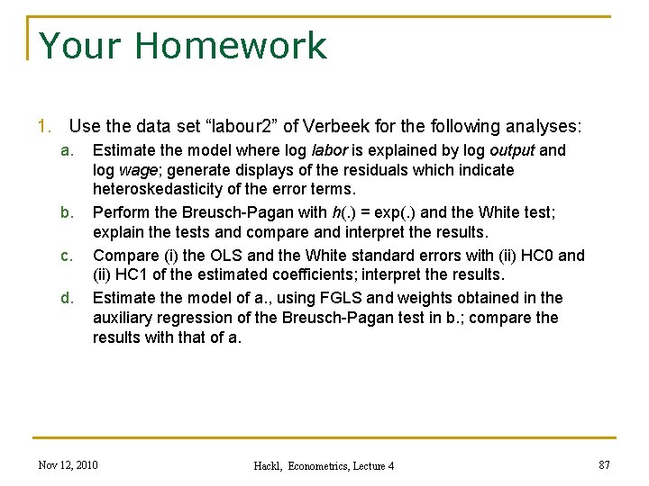
Your Homework 1. Use the data set “labour 2” of Verbeek for the following analyses: a. b. c. d. Estimate the model where log labor is explained by log output and log wage; generate displays of the residuals which indicate heteroskedasticity of the error terms. Perform the Breusch-Pagan with h(. ) = exp(. ) and the White test; explain the tests and compare and interpret the results. Compare (i) the OLS and the White standard errors with (ii) HC 0 and (ii) HC 1 of the estimated coefficients; interpret the results. Estimate the model of a. , using FGLS and weights obtained in the auxiliary regression of the Breusch-Pagan test in b. ; compare the results with that of a. Nov 12, 2010 Hackl, Econometrics, Lecture 4 87

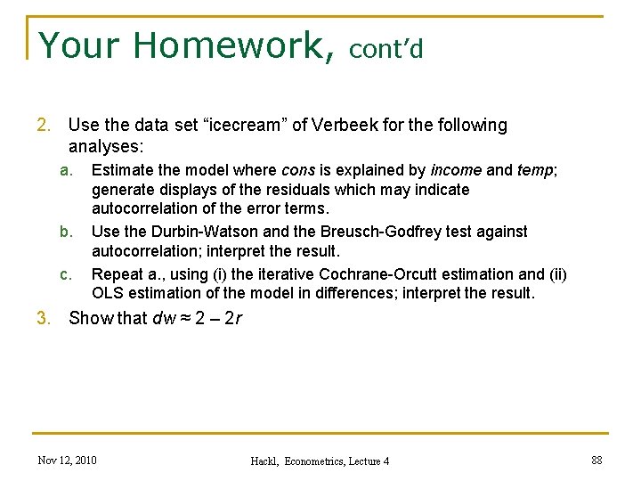
Your Homework, cont’d 2. Use the data set “icecream” of Verbeek for the following analyses: a. b. c. Estimate the model where cons is explained by income and temp; generate displays of the residuals which may indicate autocorrelation of the error terms. Use the Durbin-Watson and the Breusch-Godfrey test against autocorrelation; interpret the result. Repeat a. , using (i) the iterative Cochrane-Orcutt estimation and (ii) OLS estimation of the model in differences; interpret the result. 3. Show that dw ≈ 2 – 2 r Nov 12, 2010 Hackl, Econometrics, Lecture 4 88