Econometrics Lecture 2 Introduction to Linear Regression Part

Econometrics - Lecture 2 Introduction to Linear Regression – Part 2

Contents n n n Goodness-of-Fit Hypothesis Testing Asymptotic Properties of the OLS Estimator Multicollinearity Prediction Nov 4, 2016 Hackl, Econometrics, Lecture 2 2

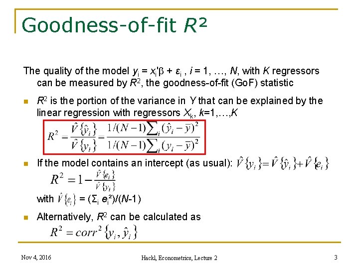
Goodness-of-fit R² The quality of the model yi = xi' + εi , i = 1, …, N, with K regressors can be measured by R 2, the goodness-of-fit (Go. F) statistic n R 2 is the portion of the variance in Y that can be explained by the linear regression with regressors Xk, k=1, …, K n If the model contains an intercept (as usual): with n = (Σi ei²)/(N-1) Alternatively, R 2 can be calculated as Nov 4, 2016 Hackl, Econometrics, Lecture 2 3

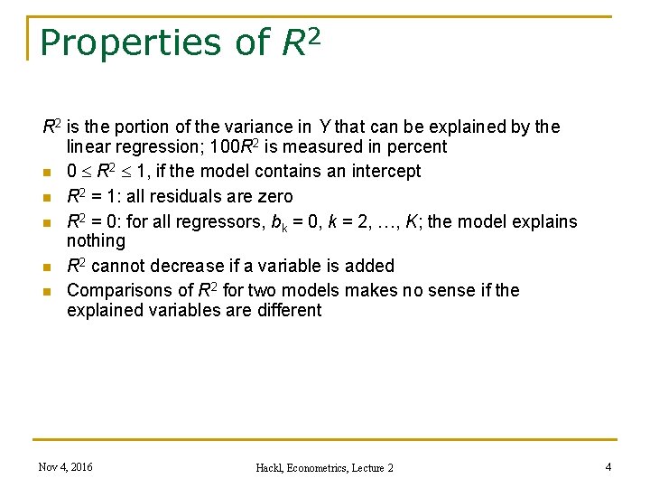
Properties of R 2 is the portion of the variance in Y that can be explained by the linear regression; 100 R 2 is measured in percent n 0 R 2 1, if the model contains an intercept n R 2 = 1: all residuals are zero n R 2 = 0: for all regressors, bk = 0, k = 2, …, K; the model explains nothing n R 2 cannot decrease if a variable is added n Comparisons of R 2 for two models makes no sense if the explained variables are different Nov 4, 2016 Hackl, Econometrics, Lecture 2 4

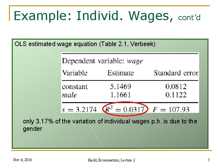
Example: Individ. Wages, cont’d OLS estimated wage equation (Table 2. 1, Verbeek) only 3. 17% of the variation of individual wages p. h. is due to the gender Nov 4, 2016 Hackl, Econometrics, Lecture 2 5

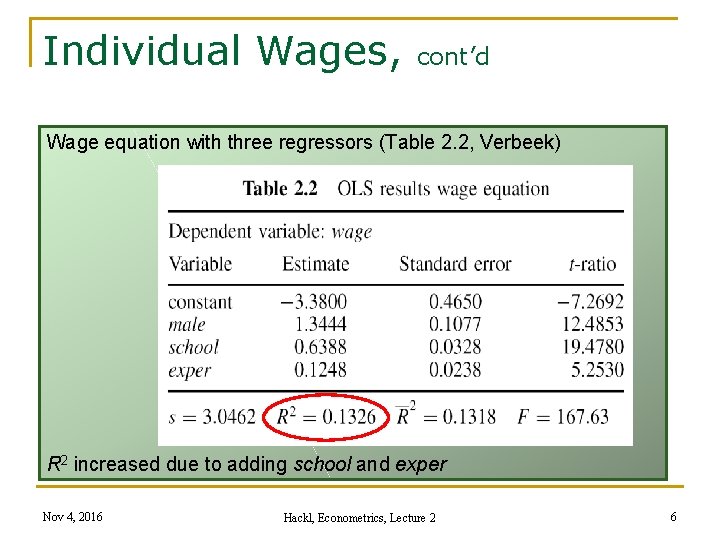
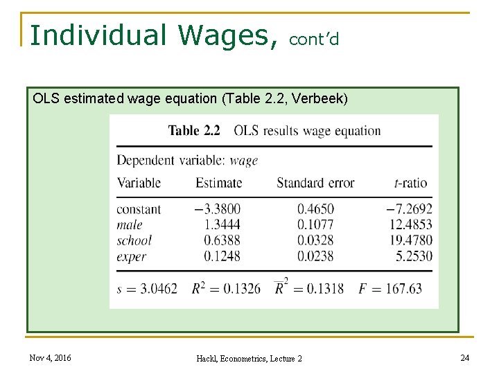
Individual Wages, cont’d Wage equation with three regressors (Table 2. 2, Verbeek) R 2 increased due to adding school and exper Nov 4, 2016 Hackl, Econometrics, Lecture 2 6

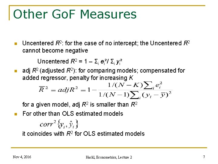
Other Go. F Measures n n n Uncentered R 2: for the case of no intercept; the Uncentered R 2 cannot become negative Uncentered R 2 = 1 – Σi ei²/ Σi yi² adj R 2 (adjusted R 2): for comparing models; compensated for added regressor, penalty for increasing K for a given model, adj R 2 is smaller than R 2 For other than OLS estimated models it coincides with R 2 for OLS estimated models Nov 4, 2016 Hackl, Econometrics, Lecture 2 7

Contents n n n Goodness-of-Fit Hypothesis Testing Asymptotic Properties of the OLS Estimator Multicollinearity Prediction Nov 4, 2016 Hackl, Econometrics, Lecture 2 8

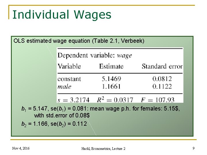
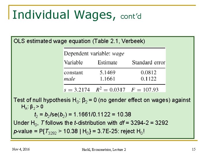
Individual Wages OLS estimated wage equation (Table 2. 1, Verbeek) b 1 = 5. 147, se(b 1) = 0. 081: mean wage p. h. for females: 5. 15$, with std. error of 0. 08$ b 2 = 1. 166, se(b 2) = 0. 112 Nov 4, 2016 Hackl, Econometrics, Lecture 2 9

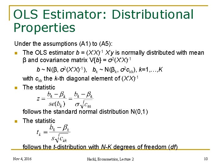
OLS Estimator: Distributional Properties Under the assumptions (A 1) to (A 5): n The OLS estimator b = (X’X)-1 X’y is normally distributed with mean β and covariance matrix V{b} = σ2(X‘X)-1 n b ~ N(β, σ2(X’X)-1), bk ~ N(βk, σ2 ckk), k=1, …, K with ckk the k-th diagonal element of (X’X)-1 The statistic n follows the standard normal distribution N(0, 1) The statistic follows the t-distribution with N-K degrees of freedom (df) Nov 4, 2016 Hackl, Econometrics, Lecture 2 10

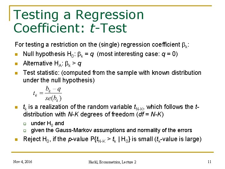
Testing a Regression Coefficient: t-Test For testing a restriction on the (single) regression coefficient k: n Null hypothesis H 0: k = q (most interesting case: q = 0) n n n Alternative HA: k > q Test statistic: (computed from the sample with known distribution under the null hypothesis) tk is a realization of the random variable t. N-K, which follows the tdistribution with N-K degrees of freedom (df = N-K) q q n under H 0 and given the Gauss-Markov assumptions and normality of the errors Reject H 0, if the p-value P{t. N-K > tk | H 0} is small (tk-value is large) Nov 4, 2016 Hackl, Econometrics, Lecture 2 11

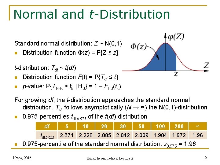
Normal and t-Distribution Standard normal distribution: Z ~ N(0, 1) n Distribution function F(z) = P{Z ≤ z} t-distribution: Tdf ~ t(df) n Distribution function F(t) = P{Tdf ≤ t} n p-value: P{TN-K > tk | H 0} = 1 – FH 0(tk) For growing df, the t-distribution approaches the standard normal distribution, Tdf follows asymptotically (N → ∞) the N(0, 1)-distribution n 0. 975 -percentiles tdf, 0. 975 of the t(df)-distribution df tdf, 0. 025 n 5 10 20 30 50 100 2. 571 2. 228 2. 085 2. 042 2. 009 1. 984 1. 972 ∞ 1. 96 0. 975 -percentile of the standard normal distribution: z 0. 975 = 1. 96 Nov 4, 2016 Hackl, Econometrics, Lecture 2 12

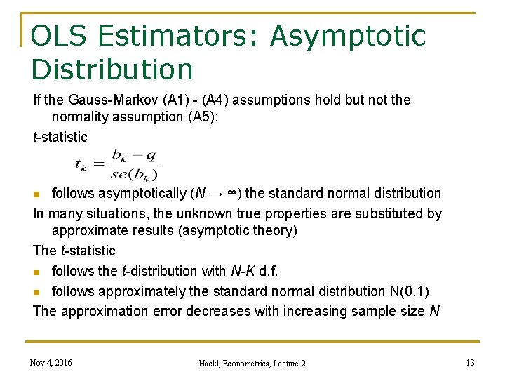
OLS Estimators: Asymptotic Distribution If the Gauss-Markov (A 1) - (A 4) assumptions hold but not the normality assumption (A 5): t-statistic follows asymptotically (N → ∞) the standard normal distribution In many situations, the unknown true properties are substituted by approximate results (asymptotic theory) The t-statistic n follows the t-distribution with N-K d. f. n follows approximately the standard normal distribution N(0, 1) The approximation error decreases with increasing sample size N n Nov 4, 2016 Hackl, Econometrics, Lecture 2 13

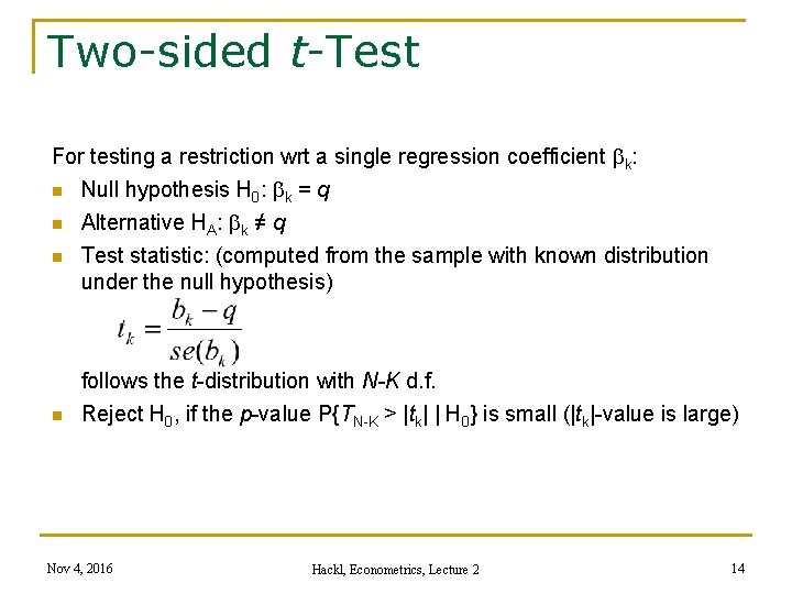
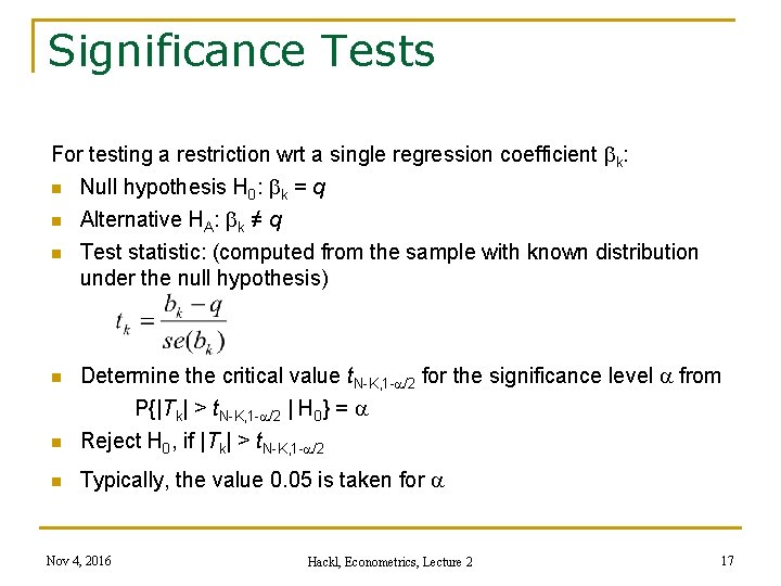
Two-sided t-Test For testing a restriction wrt a single regression coefficient k: n Null hypothesis H 0: k = q n n n Alternative HA: k ≠ q Test statistic: (computed from the sample with known distribution under the null hypothesis) follows the t-distribution with N-K d. f. Reject H 0, if the p-value P{TN-K > |tk| | H 0} is small (|tk|-value is large) Nov 4, 2016 Hackl, Econometrics, Lecture 2 14

Individual Wages, cont’d OLS estimated wage equation (Table 2. 1, Verbeek) Test of null hypothesis H 0: β 2 = 0 (no gender effect on wages) against HA: β 2 > 0 t 2 = b 2/se(b 2) = 1. 1661/0. 1122 = 10. 38 Under H 0, T follows the t-distribution with df = 3294 -2 = 3292 p-value = P{T 3292 > 10. 38 | H 0} = 3. 7 E-25: reject H 0! Nov 4, 2016 Hackl, Econometrics, Lecture 2 15

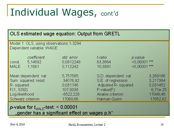
Individual Wages, cont’d OLS estimated wage equation: Output from GRETL Model 1: OLS, using observations 1 -3294 Dependent variable: WAGE const MALE coefficient 5, 14692 1, 1661 Mean dependent var Sum squared resid R- squared F(1, 3292) Log-likelihood Schwarz criterion std. error 0, 0812248 0, 112242 t-ratio 63, 3664 10, 3891 p-value <0, 00001 *** 5, 757585 34076, 92 0, 031746 107, 9338 -8522, 228 17060, 66 S. D. dependent var S. E. of regression Adjusted R- squared P-value(F) Akaike criterion Hannan-Quinn 3, 269186 3, 217364 0, 031452 6, 71 e-25 17048, 46 17052, 82 p-value for t. MALE-test: < 0. 00001 „gender has a significant effect on wages p. h“ Nov 4, 2016 Hackl, Econometrics, Lecture 2 16

Significance Tests For testing a restriction wrt a single regression coefficient k: n Null hypothesis H 0: k = q n n Alternative HA: k ≠ q Test statistic: (computed from the sample with known distribution under the null hypothesis) n Determine the critical value t. N-K, 1 -a/2 for the significance level a from P{|Tk| > t. N-K, 1 -a/2 | H 0} = a Reject H 0, if |Tk| > t. N-K, 1 -a/2 n Typically, the value 0. 05 is taken for a n Nov 4, 2016 Hackl, Econometrics, Lecture 2 17

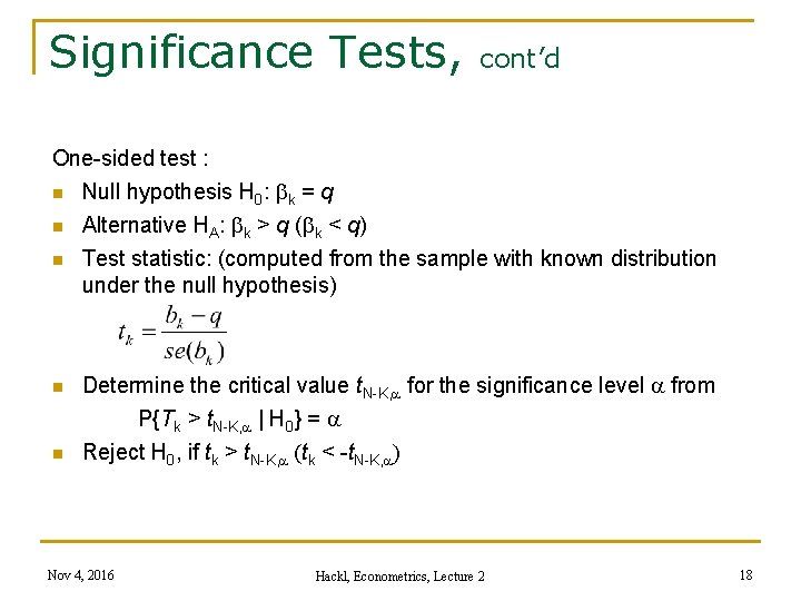
Significance Tests, cont’d One-sided test : n Null hypothesis H 0: k = q n n Alternative HA: k > q ( k < q) Test statistic: (computed from the sample with known distribution under the null hypothesis) Determine the critical value t. N-K, a for the significance level a from P{Tk > t. N-K, a | H 0} = a Reject H 0, if tk > t. N-K, a (tk < -t. N-K, a) Nov 4, 2016 Hackl, Econometrics, Lecture 2 18

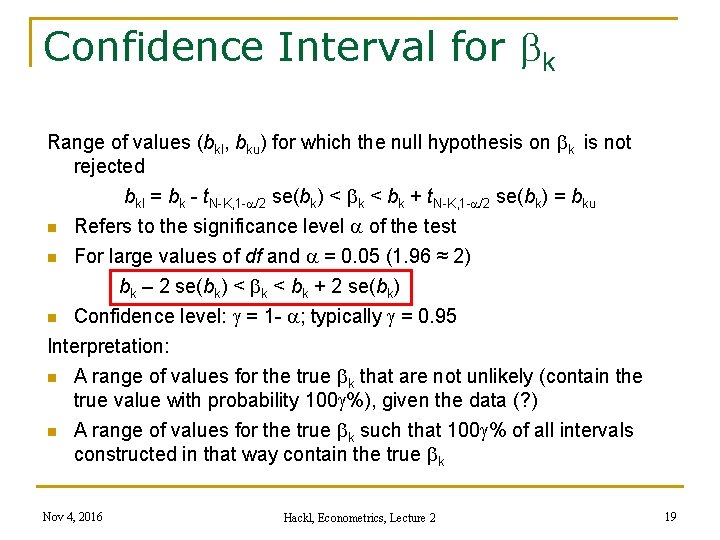
Confidence Interval for k Range of values (bkl, bku) for which the null hypothesis on k is not rejected bkl = bk - t. N-K, 1 -a/2 se(bk) < k < bk + t. N-K, 1 -a/2 se(bk) = bku n Refers to the significance level a of the test n For large values of df and a = 0. 05 (1. 96 ≈ 2) bk – 2 se(bk) < k < bk + 2 se(bk) n Confidence level: g = 1 - a; typically g = 0. 95 Interpretation: n A range of values for the true k that are not unlikely (contain the true value with probability 100 g%), given the data (? ) n A range of values for the true k such that 100 g% of all intervals constructed in that way contain the true k Nov 4, 2016 Hackl, Econometrics, Lecture 2 19

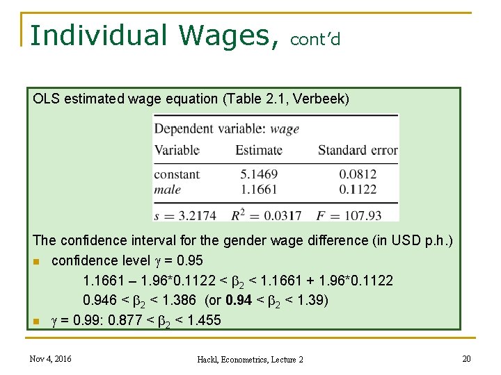
Individual Wages, cont’d OLS estimated wage equation (Table 2. 1, Verbeek) The confidence interval for the gender wage difference (in USD p. h. ) n confidence level g = 0. 95 1. 1661 – 1. 96*0. 1122 < 1. 1661 + 1. 96*0. 1122 0. 946 < 2 < 1. 386 (or 0. 94 < 2 < 1. 39) n g = 0. 99: 0. 877 < 2 < 1. 455 Nov 4, 2016 Hackl, Econometrics, Lecture 2 20

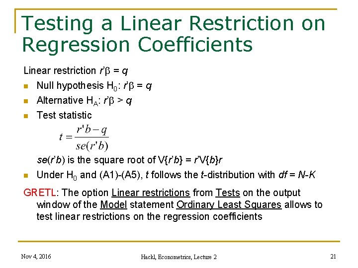
Testing a Linear Restriction on Regression Coefficients Linear restriction r’ = q n Null hypothesis H 0: r’ = q n Alternative HA: r’ > q Test statistic n se(r’b) is the square root of V{r’b} = r’V{b}r Under H 0 and (A 1)-(A 5), t follows the t-distribution with df = N-K n GRETL: The option Linear restrictions from Tests on the output window of the Model statement Ordinary Least Squares allows to test linear restrictions on the regression coefficients Nov 4, 2016 Hackl, Econometrics, Lecture 2 21

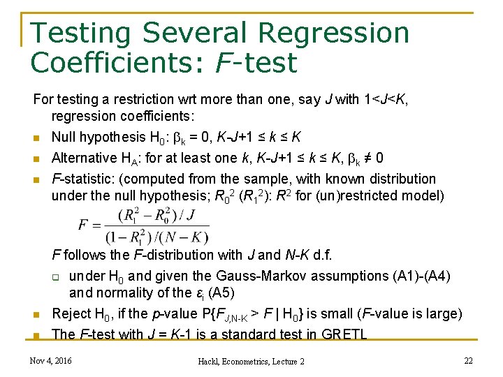
Testing Several Regression Coefficients: F-test For testing a restriction wrt more than one, say J with 1<J<K, regression coefficients: n n n Null hypothesis H 0: k = 0, K-J+1 ≤ k ≤ K Alternative HA: for at least one k, K-J+1 ≤ k ≤ K, k ≠ 0 F-statistic: (computed from the sample, with known distribution under the null hypothesis; R 02 (R 12): R 2 for (un)restricted model) F follows the F-distribution with J and N-K d. f. under H 0 and given the Gauss-Markov assumptions (A 1)-(A 4) and normality of the εi (A 5) Reject H 0, if the p-value P{FJ, N-K > F | H 0} is small (F-value is large) The F-test with J = K-1 is a standard test in GRETL q n n Nov 4, 2016 Hackl, Econometrics, Lecture 2 22

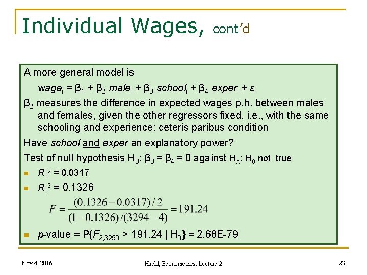
Individual Wages, cont’d A more general model is wagei = β 1 + β 2 malei + β 3 schooli + β 4 experi + εi β 2 measures the difference in expected wages p. h. between males and females, given the other regressors fixed, i. e. , with the same schooling and experience: ceteris paribus condition Have school and exper an explanatory power? Test of null hypothesis H 0: β 3 = β 4 = 0 against HA: H 0 not true n R 02 = 0. 0317 n R 12 = 0. 1326 n p-value = P{F 2, 3290 > 191. 24 | H 0} = 2. 68 E-79 Nov 4, 2016 Hackl, Econometrics, Lecture 2 23

Individual Wages, cont’d OLS estimated wage equation (Table 2. 2, Verbeek) Nov 4, 2016 Hackl, Econometrics, Lecture 2 24

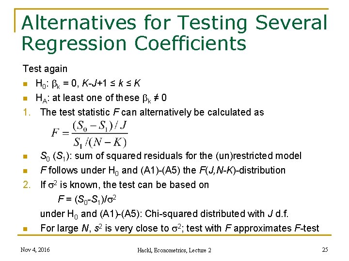
Alternatives for Testing Several Regression Coefficients Test again n H 0: k = 0, K-J+1 ≤ k ≤ K HA: at least one of these k ≠ 0 1. The test statistic F can alternatively be calculated as n n n S 0 (S 1): sum of squared residuals for the (un)restricted model F follows under H 0 and (A 1)-(A 5) the F(J, N-K)-distribution 2. If s 2 is known, the test can be based on F = (S 0 -S 1)/s 2 under H 0 and (A 1)-(A 5): Chi-squared distributed with J d. f. n For large N, s 2 is very close to s 2; test with F approximates F-test Nov 4, 2016 Hackl, Econometrics, Lecture 2 25

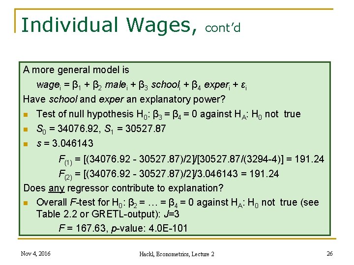
Individual Wages, cont’d A more general model is wagei = β 1 + β 2 malei + β 3 schooli + β 4 experi + εi Have school and exper an explanatory power? n Test of null hypothesis H 0: β 3 = β 4 = 0 against HA: H 0 not true n S 0 = 34076. 92, S 1 = 30527. 87 n s = 3. 046143 F(1) = [(34076. 92 - 30527. 87)/2]/[30527. 87/(3294 -4)] = 191. 24 F(2) = [(34076. 92 - 30527. 87)/2]/3. 046143 = 191. 24 Does any regressor contribute to explanation? n Overall F-test for H 0: β 2 = … = β 4 = 0 against HA: H 0 not true (see Table 2. 2 or GRETL-output): J=3 F = 167. 63, p-value: 4. 0 E-101 Nov 4, 2016 Hackl, Econometrics, Lecture 2 26

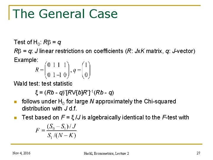
The General Case Test of H 0: R = q: J linear restrictions on coefficients (R: Jx. K matrix, q: J-vector) Example: Wald test: test statistic ξ = (Rb - q)’[RV{b}R’]-1(Rb - q) n follows under H 0 for large N approximately the Chi-squared distribution with J d. f. n Test based on F = ξ /J is algebraically identical to the F-test with Nov 4, 2016 Hackl, Econometrics, Lecture 2 27

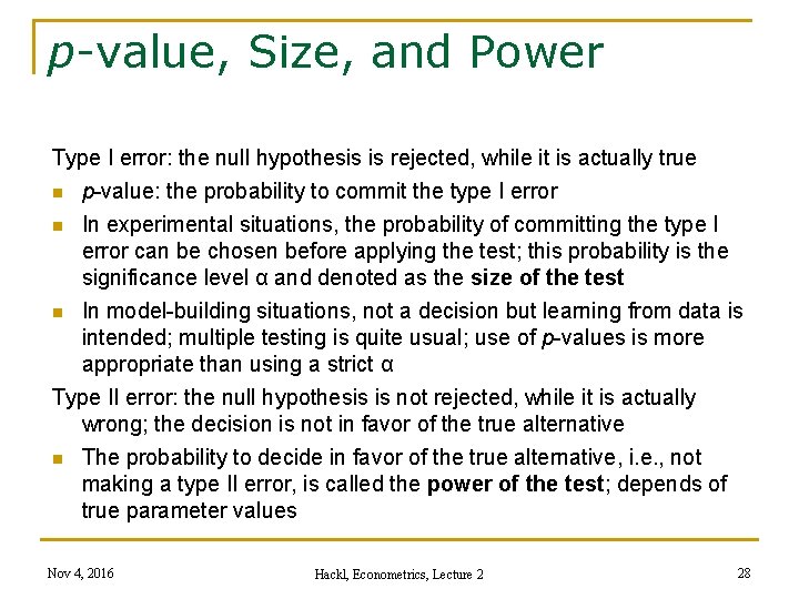
p-value, Size, and Power Type I error: the null hypothesis is rejected, while it is actually true n p-value: the probability to commit the type I error In experimental situations, the probability of committing the type I error can be chosen before applying the test; this probability is the significance level α and denoted as the size of the test n In model-building situations, not a decision but learning from data is intended; multiple testing is quite usual; use of p-values is more appropriate than using a strict α Type II error: the null hypothesis is not rejected, while it is actually wrong; the decision is not in favor of the true alternative n The probability to decide in favor of the true alternative, i. e. , not making a type II error, is called the power of the test; depends of true parameter values n Nov 4, 2016 Hackl, Econometrics, Lecture 2 28

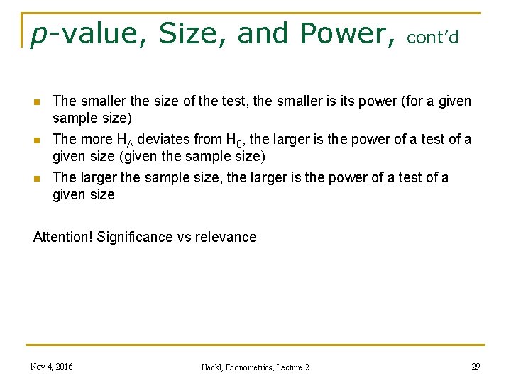
p-value, Size, and Power, cont’d n The smaller the size of the test, the smaller is its power (for a given sample size) n The more HA deviates from H 0, the larger is the power of a test of a given size (given the sample size) The larger the sample size, the larger is the power of a test of a given size n Attention! Significance vs relevance Nov 4, 2016 Hackl, Econometrics, Lecture 2 29

Contents n n n Goodness-of-Fit Hypothesis Testing Asymptotic Properties of the OLS Estimator Multicollinearity Prediction Nov 4, 2016 Hackl, Econometrics, Lecture 2 30

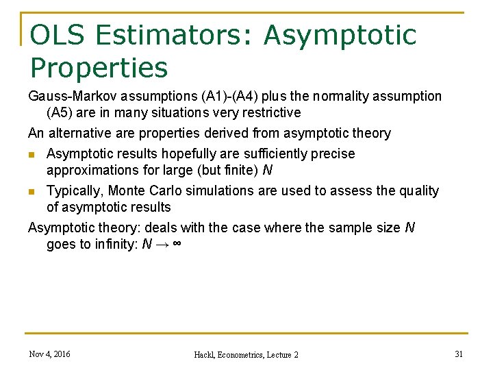
OLS Estimators: Asymptotic Properties Gauss-Markov assumptions (A 1)-(A 4) plus the normality assumption (A 5) are in many situations very restrictive An alternative are properties derived from asymptotic theory n Asymptotic results hopefully are sufficiently precise approximations for large (but finite) N n Typically, Monte Carlo simulations are used to assess the quality of asymptotic results Asymptotic theory: deals with the case where the sample size N goes to infinity: N → ∞ Nov 4, 2016 Hackl, Econometrics, Lecture 2 31

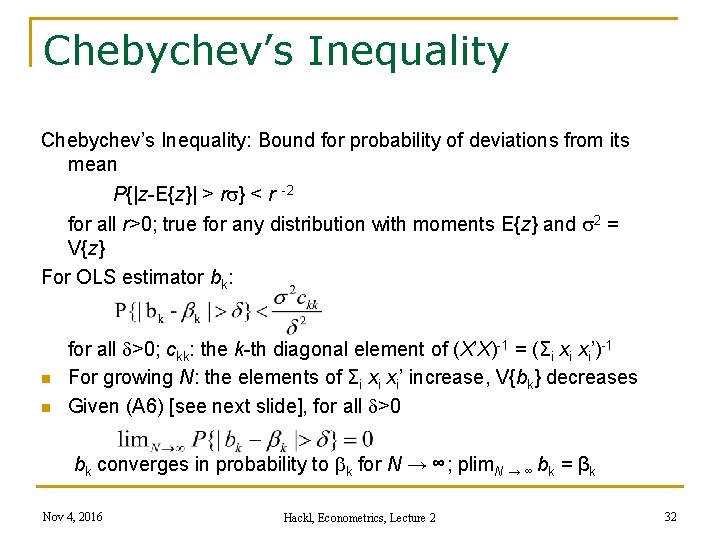
Chebychev’s Inequality: Bound for probability of deviations from its mean P{|z-E{z}| > rs} < r- -2 for all r>0; true for any distribution with moments E{z} and s 2 = V{z} For OLS estimator bk: n n for all d>0; ckk: the k-th diagonal element of (X’X)-1 = (Σi xi xi’)-1 For growing N: the elements of Σi xi xi’ increase, V{bk} decreases Given (A 6) [see next slide], for all d>0 bk converges in probability to k for N → ∞; plim. N → ∞ bk = βk Nov 4, 2016 Hackl, Econometrics, Lecture 2 32

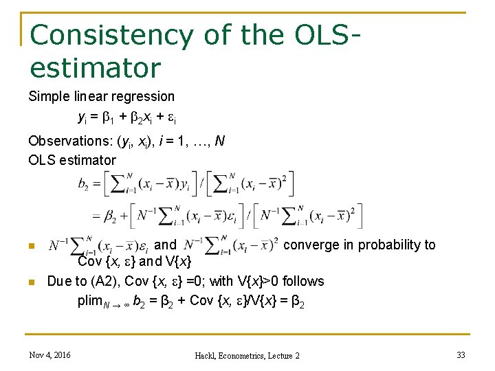
Consistency of the OLSestimator Simple linear regression yi = 1 + 2 xi + ei Observations: (yi, xi), i = 1, …, N OLS estimator n n and converge in probability to Cov {x, e} and V{x} Due to (A 2), Cov {x, e} =0; with V{x}>0 follows plim. N → ∞ b 2 = β 2 + Cov {x, e}/V{x} = β 2 Nov 4, 2016 Hackl, Econometrics, Lecture 2 33

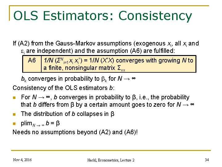
OLS Estimators: Consistency If (A 2) from the Gauss-Markov assumptions (exogenous xi, all xi and ei are independent) and the assumption (A 6) are fulfilled: A 6 1/N (ΣNi=1 xi xi’) = 1/N (X’X) converges with growing N to a finite, nonsingular matrix Σxx bk converges in probability to k for N → ∞ Consistency of the OLS estimators b: n For N → ∞, b converges in probability to β, i. e. , the probability that b differs from β by a certain amount goes to zero for N → ∞ n The distribution of b collapses in β n plim. N → ∞ b = β Needs no assumptions beyond (A 2) and (A 6)! Nov 4, 2016 Hackl, Econometrics, Lecture 2 34

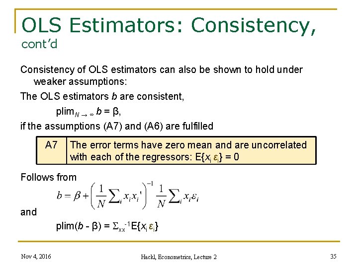
OLS Estimators: Consistency, cont’d Consistency of OLS estimators can also be shown to hold under weaker assumptions: The OLS estimators b are consistent, plim. N → ∞ b = β, if the assumptions (A 7) and (A 6) are fulfilled A 7 The error terms have zero mean and are uncorrelated with each of the regressors: E{xi εi} = 0 Follows from and plim(b - β) = Sxx-1 E{xi εi} Nov 4, 2016 Hackl, Econometrics, Lecture 2 35

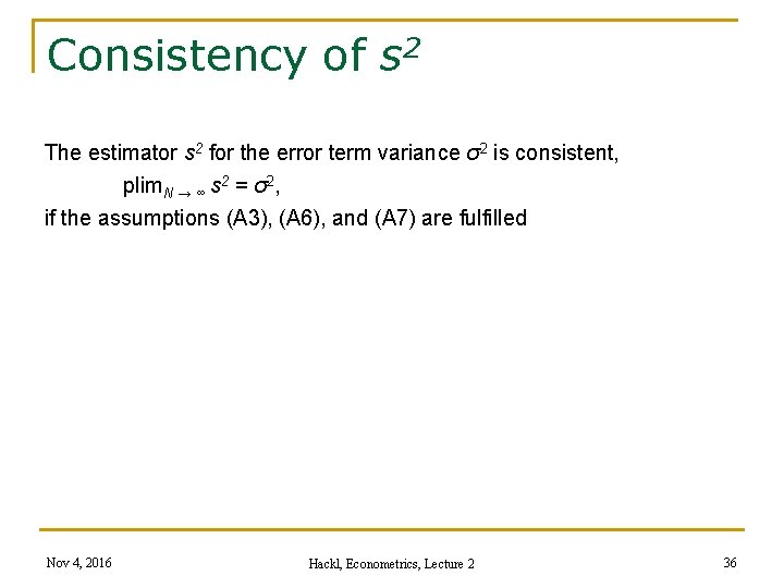
Consistency of s 2 The estimator s 2 for the error term variance σ2 is consistent, plim. N → ∞ s 2 = σ2, if the assumptions (A 3), (A 6), and (A 7) are fulfilled Nov 4, 2016 Hackl, Econometrics, Lecture 2 36

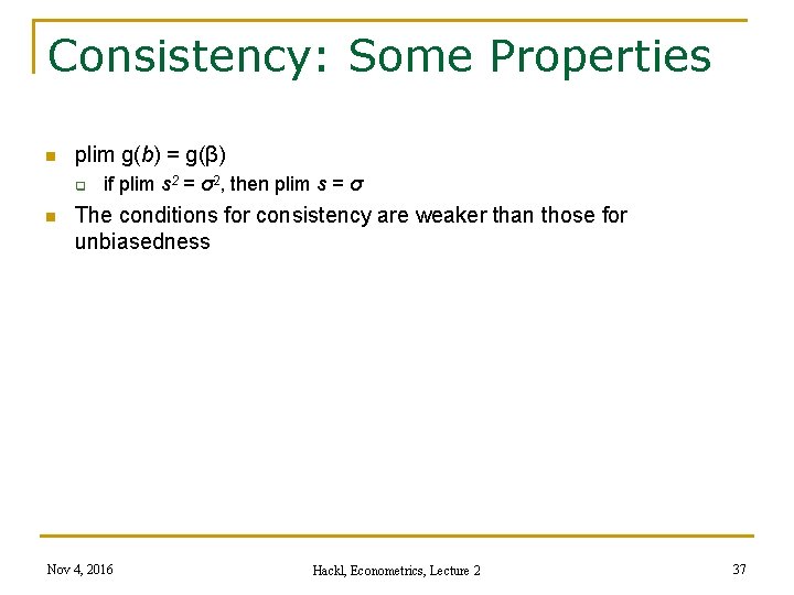
Consistency: Some Properties n plim g(b) = g(β) q n if plim s 2 = σ2, then plim s = σ The conditions for consistency are weaker than those for unbiasedness Nov 4, 2016 Hackl, Econometrics, Lecture 2 37

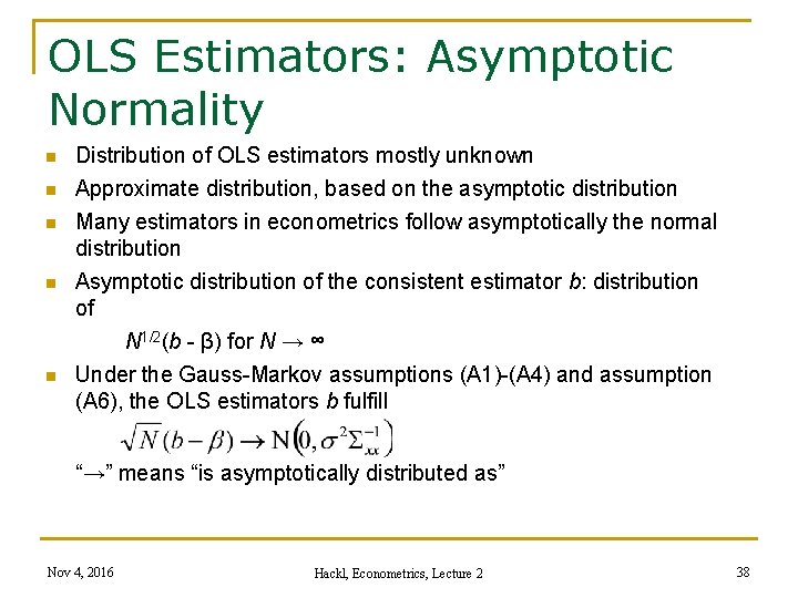
OLS Estimators: Asymptotic Normality n n n Distribution of OLS estimators mostly unknown Approximate distribution, based on the asymptotic distribution Many estimators in econometrics follow asymptotically the normal distribution Asymptotic distribution of the consistent estimator b: distribution of N 1/2(b - β) for N → ∞ Under the Gauss-Markov assumptions (A 1)-(A 4) and assumption (A 6), the OLS estimators b fulfill “→” means “is asymptotically distributed as” Nov 4, 2016 Hackl, Econometrics, Lecture 2 38

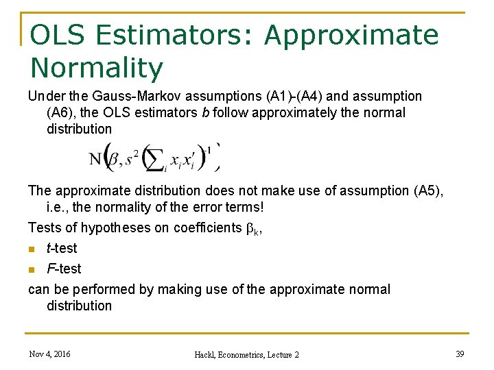
OLS Estimators: Approximate Normality Under the Gauss-Markov assumptions (A 1)-(A 4) and assumption (A 6), the OLS estimators b follow approximately the normal distribution The approximate distribution does not make use of assumption (A 5), i. e. , the normality of the error terms! Tests of hypotheses on coefficients k, n t-test n F-test can be performed by making use of the approximate normal distribution Nov 4, 2016 Hackl, Econometrics, Lecture 2 39

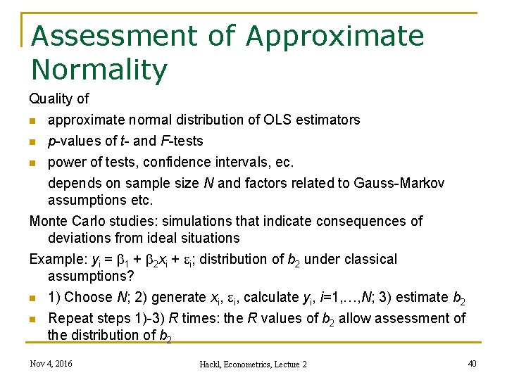
Assessment of Approximate Normality Quality of n approximate normal distribution of OLS estimators p-values of t- and F-tests n power of tests, confidence intervals, ec. depends on sample size N and factors related to Gauss-Markov assumptions etc. Monte Carlo studies: simulations that indicate consequences of deviations from ideal situations Example: yi = 1 + 2 xi + ei; distribution of b 2 under classical assumptions? n 1) Choose N; 2) generate xi, ei, calculate yi, i=1, …, N; 3) estimate b 2 n Repeat steps 1)-3) R times: the R values of b 2 allow assessment of the distribution of b 2 n Nov 4, 2016 Hackl, Econometrics, Lecture 2 40

Contents n n n Goodness-of-Fit Hypothesis Testing Asymptotic Properties of the OLS Estimator Multicollinearity Prediction Nov 4, 2016 Hackl, Econometrics, Lecture 2 41

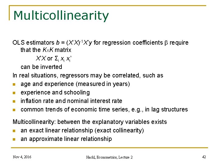
Multicollinearity OLS estimators b = (X’X)-1 X’y for regression coefficients require that the Kx. K matrix X’X or Σi xi xi’ can be inverted In real situations, regressors may be correlated, such as n age and experience (measured in years) n experience and schooling n inflation rate and nominal interest rate n common trends of economic time series, e. g. , in lag structures Multicollinearity: between the explanatory variables exists n an exact linear relationship (exact collinearity) n an approximate linear relationship Nov 4, 2016 Hackl, Econometrics, Lecture 2 42

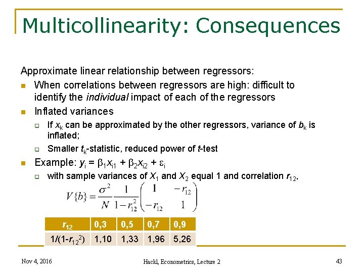
Multicollinearity: Consequences Approximate linear relationship between regressors: n When correlations between regressors are high: difficult to identify the individual impact of each of the regressors n Inflated variances q q n If xk can be approximated by the other regressors, variance of bk is inflated; Smaller tk-statistic, reduced power of t-test Example: yi = 1 xi 1 + 2 xi 2 + ei q with sample variances of X 1 and X 2 equal 1 and correlation r 12, r 12 1/(1 -r 122) Nov 4, 2016 0, 3 0, 5 0, 7 0, 9 1, 10 1, 33 1, 96 5, 26 Hackl, Econometrics, Lecture 2 43

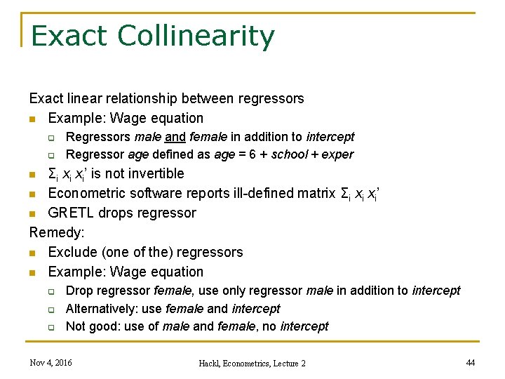
Exact Collinearity Exact linear relationship between regressors n Example: Wage equation q q Regressors male and female in addition to intercept Regressor age defined as age = 6 + school + exper Σi xi xi’ is not invertible n Econometric software reports ill-defined matrix Σi xi xi’ n GRETL drops regressor Remedy: n Exclude (one of the) regressors n Example: Wage equation n q q q Drop regressor female, use only regressor male in addition to intercept Alternatively: use female and intercept Not good: use of male and female, no intercept Nov 4, 2016 Hackl, Econometrics, Lecture 2 44

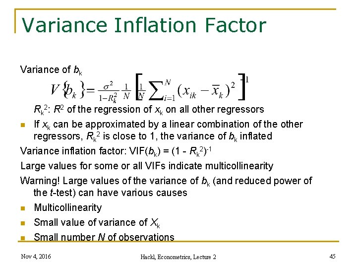
Variance Inflation Factor Variance of bk Rk 2: R 2 of the regression of xk on all other regressors n If xk can be approximated by a linear combination of the other regressors, Rk 2 is close to 1, the variance of bk inflated Variance inflation factor: VIF(bk) = (1 - Rk 2)-1 Large values for some or all VIFs indicate multicollinearity Warning! Large values of the variance of bk (and reduced power of the t-test) can have various causes n Multicollinearity n Small value of variance of Xk n Small number N of observations Nov 4, 2016 Hackl, Econometrics, Lecture 2 45

Other Indicators for Multicollinearity Large values for some or all variance inflation factors VIF(bk) are an indicator for multicollinearity Other indicators: n At least one of the Rk 2, k = 1, …, K, has a large value n Large values of standard errors se(bk) (low t-statistics), but reasonable or good R 2 and F-statistic n Effect of adding a regressor on standard errors se(bk) of estimates bk of regressors already in the model: increasing values of se(bk) indicate multicollinearity Nov 4, 2016 Hackl, Econometrics, Lecture 2 46

Contents n n n Goodness-of-Fit Hypothesis Testing Asymptotic Properties of the OLS Estimator Multicollinearity Prediction Nov 4, 2016 Hackl, Econometrics, Lecture 2 47

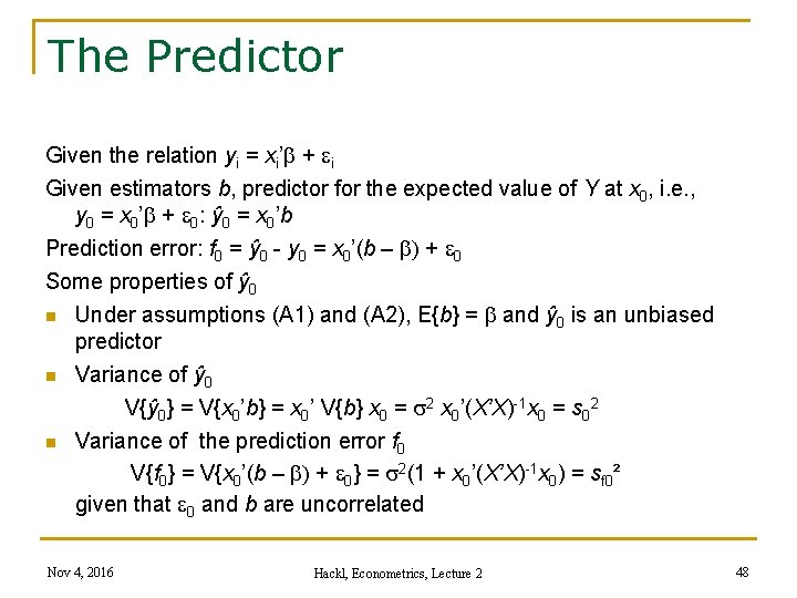
The Predictor Given the relation yi = xi’ + ei Given estimators b, predictor for the expected value of Y at x 0, i. e. , y 0 = x 0’ + e 0: ŷ 0 = x 0’b Prediction error: f 0 = ŷ 0 - y 0 = x 0’(b – ) + e 0 Some properties of ŷ 0 n Under assumptions (A 1) and (A 2), E{b} = and ŷ 0 is an unbiased predictor n Variance of ŷ 0 V{ŷ 0} = V{x 0’b} = x 0’ V{b} x 0 = s 2 x 0’(X’X)-1 x 0 = s 02 n Variance of the prediction error f 0 V{f 0} = V{x 0’(b – ) + e 0} = s 2(1 + x 0’(X’X)-1 x 0) = sf 0² given that e 0 and b are uncorrelated Nov 4, 2016 Hackl, Econometrics, Lecture 2 48

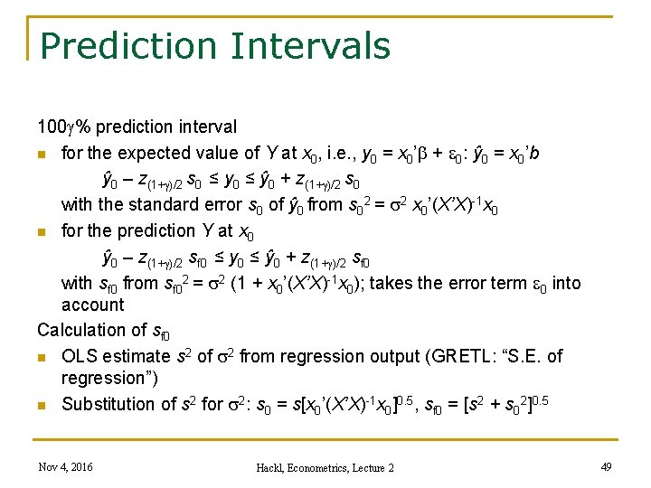
Prediction Intervals 100 g% prediction interval n for the expected value of Y at x 0, i. e. , y 0 = x 0’ + e 0: ŷ 0 = x 0’b ŷ 0 – z(1+g)/2 s 0 ≤ y 0 ≤ ŷ 0 + z(1+g)/2 s 0 with the standard error s 0 of ŷ 0 from s 02 = s 2 x 0’(X’X)-1 x 0 n for the prediction Y at x 0 ŷ 0 – z(1+g)/2 sf 0 ≤ y 0 ≤ ŷ 0 + z(1+g)/2 sf 0 with sf 0 from sf 02 = s 2 (1 + x 0’(X’X)-1 x 0); takes the error term e 0 into account Calculation of sf 0 n OLS estimate s 2 of s 2 from regression output (GRETL: “S. E. of regression”) n Substitution of s 2 for s 2: s 0 = s[x 0’(X’X)-1 x 0]0. 5, sf 0 = [s 2 + s 02]0. 5 Nov 4, 2016 Hackl, Econometrics, Lecture 2 49

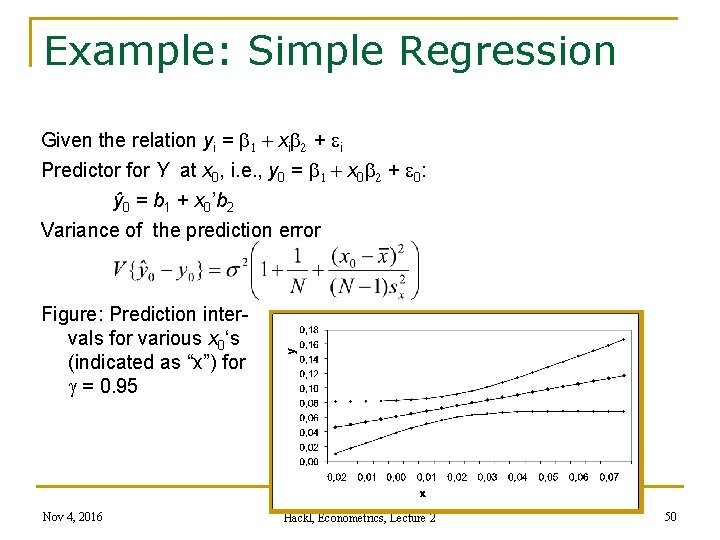
Example: Simple Regression Given the relation yi = 1 + xi 2 + ei Predictor for Y at x 0, i. e. , y 0 = 1 + x 0 2 + e 0: ŷ 0 = b 1 + x 0’b 2 Variance of the prediction error Figure: Prediction intervals for various x 0‘s (indicated as “x”) for g = 0. 95 Nov 4, 2016 Hackl, Econometrics, Lecture 2 50

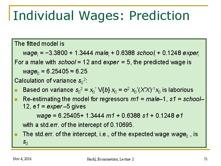
Individual Wages: Prediction The fitted model is wagei = − 3. 3800 + 1. 3444 malei + 0. 6388 schooli + 0. 1248 experi For a male with school = 12 and exper = 5, the predicted wage is wage 0 = 6. 25405 ≈ 6. 25 Calculation of variance s 02: n Based on variance s 02 = x 0’ V{b} x 0 = s 2 x 0’(X’X)-1 x 0 is laborious n Re-estimating the model for regressors m 1 = male– 1, s 1 = school– 12, e 1 = exper – 5 gives wage = 6. 25405+ 1. 3444 m 1 + 0. 6388 s 1 + 0. 1248 e 1 with a std. err. of the intercept of 0. 10695. n The std. err. of the intercept, i. e. , of the expected wage 0 , is s 0 Nov 4, 2016 Hackl, Econometrics, Lecture 2 51

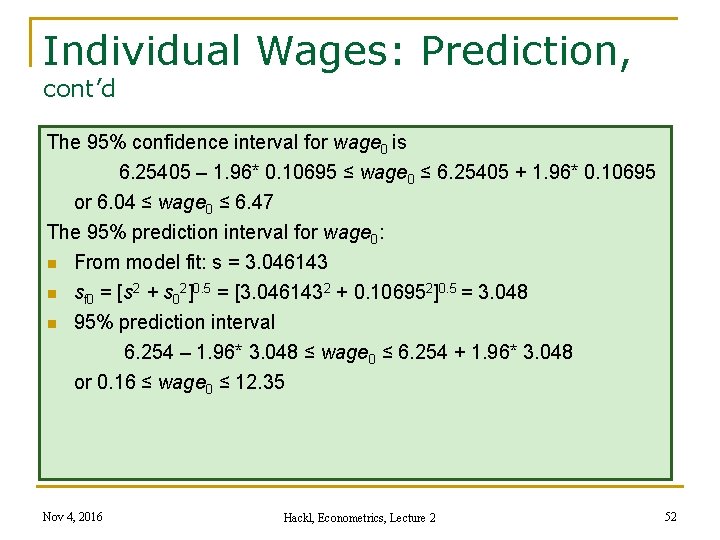
Individual Wages: Prediction, cont’d The 95% confidence interval for wage 0 is 6. 25405 – 1. 96* 0. 10695 ≤ wage 0 ≤ 6. 25405 + 1. 96* 0. 10695 or 6. 04 ≤ wage 0 ≤ 6. 47 The 95% prediction interval for wage 0: n From model fit: s = 3. 046143 n sf 0 = [s 2 + s 02]0. 5 = [3. 0461432 + 0. 106952]0. 5 = 3. 048 n 95% prediction interval 6. 254 – 1. 96* 3. 048 ≤ wage 0 ≤ 6. 254 + 1. 96* 3. 048 or 0. 16 ≤ wage 0 ≤ 12. 35 Nov 4, 2016 Hackl, Econometrics, Lecture 2 52

Your Homework 1. For Verbeek’s data set “wages 1” use GRETL (a) for estimating a linear regression model with intercept for wage p. h. with explanatory variables male and school; (b) interpret the coefficients of the model; (c) test the hypothesis that men and women, on average, have the same wage p. h. , against the alternative that women‘s wage p. h. are different from men’s wage p. h. ; (d) repeat this test against the alternative that women earn less; (e) calculate a 95% confidence interval for the wage difference of males and females. 2. Generate a variable exper_b by adding the Binomial random variable BE~B(2, 0. 5) to exper; (a) estimate two linear regression models with intercept for wage p. h. with explanatory variables (i) male and exper, and (ii) male, exper_b, and exper; compare the standard errors of the estimated coefficients; Nov 4, 2016 Hackl, Econometrics, Lecture 2 53

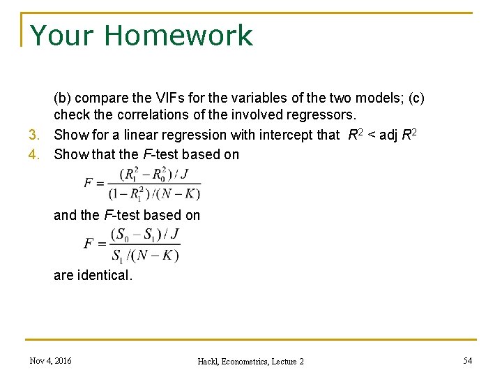
Your Homework (b) compare the VIFs for the variables of the two models; (c) check the correlations of the involved regressors. 3. Show for a linear regression with intercept that R 2 < adj R 2 4. Show that the F-test based on and the F-test based on are identical. Nov 4, 2016 Hackl, Econometrics, Lecture 2 54