Chapter 2 Simple linear regression model Definition of

Chapter 2 Simple linear regression model

Definition of the simple regression model • Much of the applied econometrics analysis begins with the following premises: y and x are two variables, representing some population, and we are interested in explaining y in terms of x or in studying how y varies with the changes in x. • In writing down a model that will explain y in terms of x, we must confront three issues. 1. Since there is never an exact relationship between two variables, how do we allow other factors to affect y? 2. What is the functional relationship between y and x? 3. How can we be sure we are capturing a ceteris paribus relationship between y and x?

Definition of the simple regression model •

THE CONCEPT OF POPULATION REGRESSION FUNІCTION (PRF) E(Y | Xi) = f (Xi) is known as conditional expectation function(CEF) or population regression function (PRF) or population regression (PR) for short. In simple terms, it tells how the mean or average of response of Y varies with X. E(Y)= f(Xi) is known as unconditional mean or unconditional expected value WHICH ONE WILL YOU PREFER?

80 100 120 140 160 180 200 220 240 260 55 65 79 80 102 110 120 135 137 150 Weekly family consumption expenditure Y, $ 60 70 84 93 107 115 136 137 145 152 65 74 90 95 110 120 140 155 175 70 80 94 103 116 130 144 152 165 178 75 85 98 108 118 135 145 157 175 180 – 113 125 140 – 160 189 185 – 88 – – – 115 – – – 162 – 191 325 462 445 707 678 750 685 1043 966 1211 Conditional means 65 of Y E (Y | X ) 77 101 113 125 137 149 161 173 Total 89

The dark circled points in the figure below show the conditional mean values of Y against the various X values. If we join these conditional mean values, we obtain what is known as population regression line or population regression curve

THE CONCEPT OF POPULATION REGRESSION FUNІCTION (PRF) •

The meaning of the term linear •

The meaning of the term linear •

The meaning of the term linear Linearity in the parameters Therefore, from now on the term “linear” regression will always mean a regression that is linear in the parameters; the β ’s (that is, the parameters are raised to the first power only). It may or may not be linear in the explanatory variables.

The meaning of the term linear •

Stochastic Specification for PRF •

Stochastic Specification for PRF The significance of stochastic disturbance term 1. Vagueness of theory 2. Unavailability of data 3. Core variable versus peripheral variables 4. Intrinsic randomness in human behavior 5. Poor proxy variables 6. Principle of parsimony 7. Wrong functional form

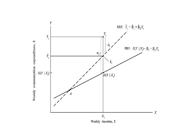
The Sample Regression Function (SRF) • By confining our discussion so far to the population of Y values corresponding to the fixed X’s, we have deliberately avoided sampling considerations. • It is about time to face up to the sampling problems, for in most practical situations what we have is but a sample of Y values corresponding to some fixed X’s. • Therefore, our task now is to estimate the PRF on the basis of the sample information.

The Sample Regression Function (SRF) As an illustration, pretend that the population in the table in the slide above was not known to us and the only information we had was a randomly selected sample of Y values for the fixed X’s as given in the table in the next slide.

The Sample Regression Function (SRF) Y 70 X 65 80 100 90 120 95 140 110 160 115 180 120 200 140 220 155 240 150 260 Y X

The Sample Regression Function (SRF) 200 Weekly consumption expenditure, $ Regression based on the second sample × First sample (Table 2. 4) Second sample (Table 2. 5) SRF 2 × SRF 1 150 × 100 × × 80 100 × × × Regressio n based on the first sample × 50 120 140 160 Weekly 180 200 income, 220 240 260

The Sample Regression Function (SRF) •

The Sample Regression Function (SRF) •

The Sample Regression Function (SRF) •