Chapter 6 Multivariate models Introductory Econometrics for Finance

Chapter 6 Multivariate models ‘Introductory Econometrics for Finance’ © Chris Brooks 2002 1

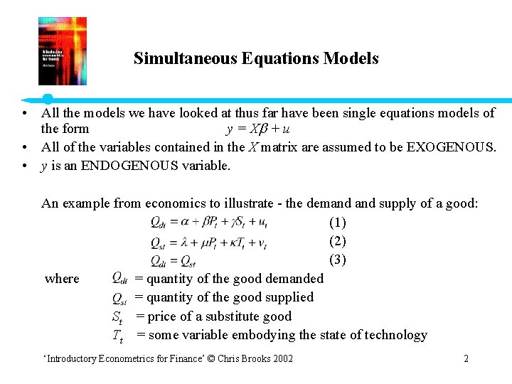
Simultaneous Equations Models • All the models we have looked at thus far have been single equations models of the form y = X + u • All of the variables contained in the X matrix are assumed to be EXOGENOUS. • y is an ENDOGENOUS variable. An example from economics to illustrate - the demand supply of a good: (1) (2) (3) where = quantity of the good demanded = quantity of the good supplied St = price of a substitute good Tt = some variable embodying the state of technology ‘Introductory Econometrics for Finance’ © Chris Brooks 2002 2

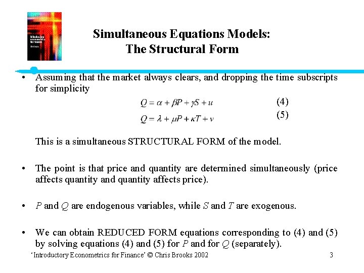
Simultaneous Equations Models: The Structural Form • Assuming that the market always clears, and dropping the time subscripts for simplicity (4) (5) This is a simultaneous STRUCTURAL FORM of the model. • The point is that price and quantity are determined simultaneously (price affects quantity and quantity affects price). • P and Q are endogenous variables, while S and T are exogenous. • We can obtain REDUCED FORM equations corresponding to (4) and (5) by solving equations (4) and (5) for P and for Q (separately). ‘Introductory Econometrics for Finance’ © Chris Brooks 2002 3

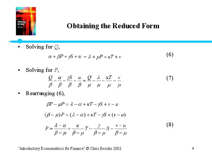
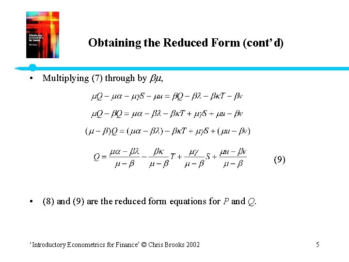
Obtaining the Reduced Form • Solving for Q, (6) • Solving for P, (7) • Rearranging (6), (8) ‘Introductory Econometrics for Finance’ © Chris Brooks 2002 4

Obtaining the Reduced Form (cont’d) • Multiplying (7) through by , (9) • (8) and (9) are the reduced form equations for P and Q. ‘Introductory Econometrics for Finance’ © Chris Brooks 2002 5

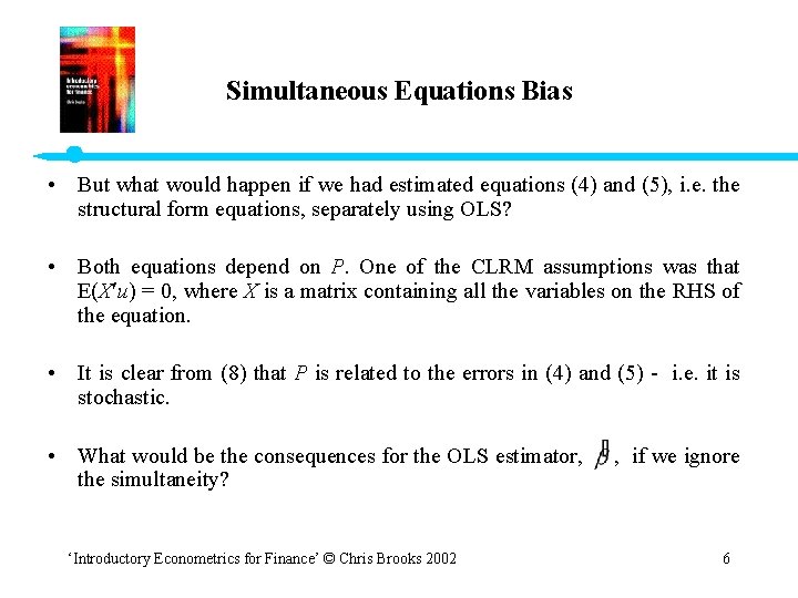
Simultaneous Equations Bias • But what would happen if we had estimated equations (4) and (5), i. e. the structural form equations, separately using OLS? • Both equations depend on P. One of the CLRM assumptions was that E(X u) = 0, where X is a matrix containing all the variables on the RHS of the equation. • It is clear from (8) that P is related to the errors in (4) and (5) - i. e. it is stochastic. • What would be the consequences for the OLS estimator, , if we ignore the simultaneity? ‘Introductory Econometrics for Finance’ © Chris Brooks 2002 6

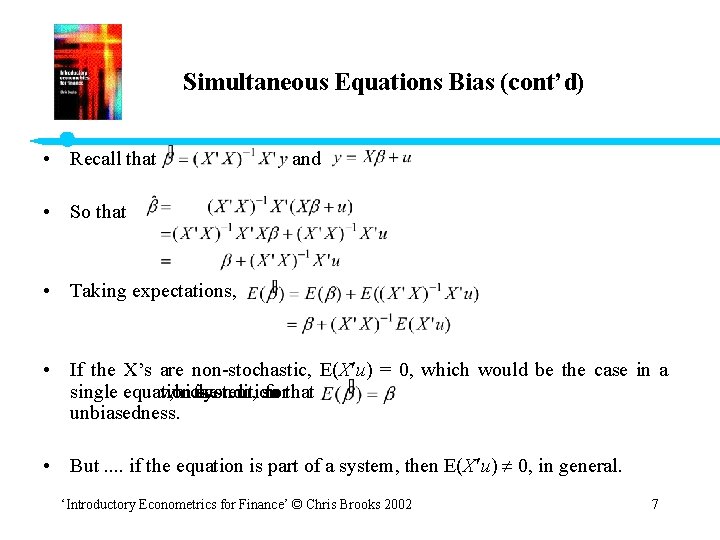
Simultaneous Equations Bias (cont’d) • Recall that • So that and • Taking expectations, • If the X’s are non-stochastic, E(X u) = 0, which would be the case in a single equation system, so that which , the is condition for unbiasedness. • But. . if the equation is part of a system, then E(X u) 0, in general. ‘Introductory Econometrics for Finance’ © Chris Brooks 2002 7

Simultaneous Equations Bias (cont’d) • Conclusion: Application of OLS to structural equations which are part of a simultaneous system will lead to biased coefficient estimates. • Is the OLS estimator still consistent, even though it is biased? • No - In fact the estimator is inconsistent as well. • Hence it would not be possible to estimate equations (4) and (5) validly using OLS. ‘Introductory Econometrics for Finance’ © Chris Brooks 2002 8

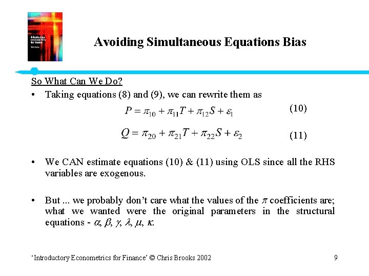
Avoiding Simultaneous Equations Bias So What Can We Do? • Taking equations (8) and (9), we can rewrite them as (10) (11) • We CAN estimate equations (10) & (11) using OLS since all the RHS variables are exogenous. • But. . . we probably don’t care what the values of the coefficients are; what we wanted were the original parameters in the structural equations - , , , . ‘Introductory Econometrics for Finance’ © Chris Brooks 2002 9

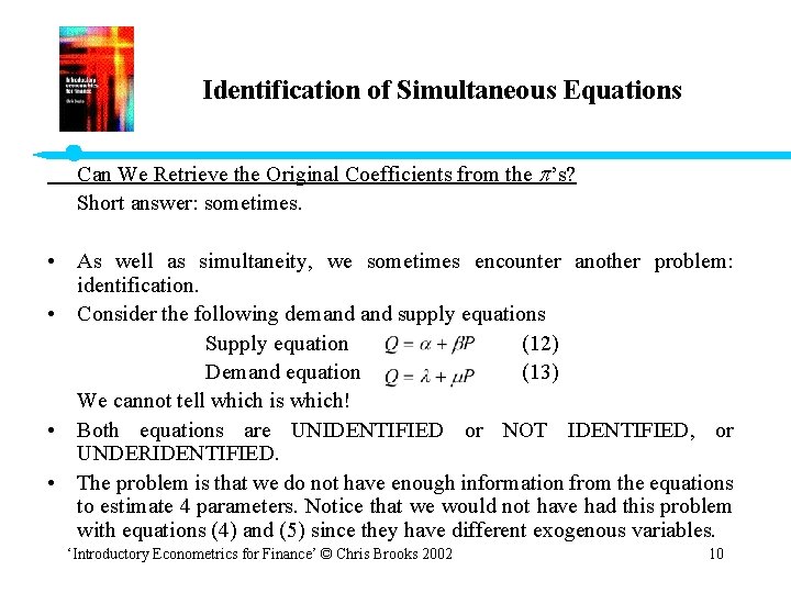
Identification of Simultaneous Equations Can We Retrieve the Original Coefficients from the ’s? Short answer: sometimes. • As well as simultaneity, we sometimes encounter another problem: identification. • Consider the following demand supply equations Supply equation (12) Demand equation (13) We cannot tell which is which! • Both equations are UNIDENTIFIED or NOT IDENTIFIED, or UNDERIDENTIFIED. • The problem is that we do not have enough information from the equations to estimate 4 parameters. Notice that we would not have had this problem with equations (4) and (5) since they have different exogenous variables. ‘Introductory Econometrics for Finance’ © Chris Brooks 2002 10

What Determines whether an Equation is Identified or not? • We could have three possible situations: 1. An equation is unidentified · like (12) or (13) · we cannot get the structural coefficients from the reduced form estimates 2. An equation is exactly identified · e. g. (4) or (5) · can get unique structural form coefficient estimates 3. An equation is over-identified · Example given later · More than one set of structural coefficients could be obtained from the reduced form. ‘Introductory Econometrics for Finance’ © Chris Brooks 2002 11

What Determines whether an Equation is Identified or not? (cont’d) • How do we tell if an equation is identified or not? • There are two conditions we could look at: - The order condition - is a necessary but not sufficient condition for an equation to be identified. - The rank condition - is a necessary and sufficient condition for identification. We specify the structural equations in a matrix form and consider the rank of a coefficient matrix. ‘Introductory Econometrics for Finance’ © Chris Brooks 2002 12

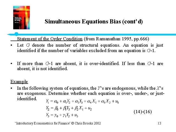
Simultaneous Equations Bias (cont’d) Statement of the Order Condition (from Ramanathan 1995, pp. 666) • Let G denote the number of structural equations. An equation is just identified if the number of variables excluded from an equation is G-1. • If more than G-1 are absent, it is over-identified. If less than G-1 are absent, it is not identified. Example • In the following system of equations, the Y’s are endogenous, while the X’s are exogenous. Determine whether each equation is over-, under-, or justidentified. (14)-(16) ‘Introductory Econometrics for Finance’ © Chris Brooks 2002 13

Simultaneous Equations Bias (cont’d) Solution G = 3; If # excluded variables = 2, the eqn is just identified If # excluded variables > 2, the eqn is over-identified If # excluded variables < 2, the eqn is not identified Equation 14: Not identified Equation 15: Just identified Equation 16: Over-identified ‘Introductory Econometrics for Finance’ © Chris Brooks 2002 14

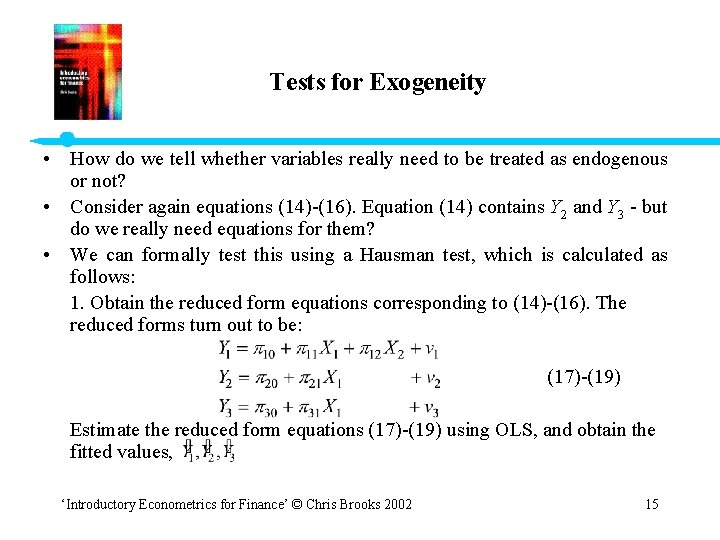
Tests for Exogeneity • How do we tell whether variables really need to be treated as endogenous or not? • Consider again equations (14)-(16). Equation (14) contains Y 2 and Y 3 - but do we really need equations for them? • We can formally test this using a Hausman test, which is calculated as follows: 1. Obtain the reduced form equations corresponding to (14)-(16). The reduced forms turn out to be: (17)-(19) Estimate the reduced form equations (17)-(19) using OLS, and obtain the fitted values, ‘Introductory Econometrics for Finance’ © Chris Brooks 2002 15

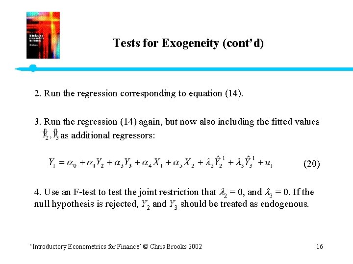
Tests for Exogeneity (cont’d) 2. Run the regression corresponding to equation (14). 3. Run the regression (14) again, but now also including the fitted values as additional regressors: (20) 4. Use an F-test to test the joint restriction that 2 = 0, and 3 = 0. If the null hypothesis is rejected, Y 2 and Y 3 should be treated as endogenous. ‘Introductory Econometrics for Finance’ © Chris Brooks 2002 16

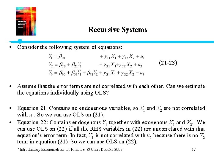
Recursive Systems • Consider the following system of equations: (21 -23) • Assume that the error terms are not correlated with each other. Can we estimate the equations individually using OLS? • Equation 21: Contains no endogenous variables, so X 1 and X 2 are not correlated with u 1. So we can use OLS on (21). • Equation 22: Contains endogenous Y 1 together with exogenous X 1 and X 2. We can use OLS on (22) if all the RHS variables in (22) are uncorrelated with that equation’s error term. In fact, Y 1 is not correlated with u 2 because there is no Y 2 term in equation (21). So we can use OLS on (22). ‘Introductory Econometrics for Finance’ © Chris Brooks 2002 17

Recursive Systems (cont’d) • Equation 23: Contains both Y 1 and Y 2; we require these to be uncorrelated with u 3. By similar arguments to the above, equations (21) and (22) do not contain Y 3, so we can use OLS on (23). • This is known as a RECURSIVE or TRIANGULAR system. We do not have a simultaneity problem here. • But in practice not many systems of equations will be recursive. . . ‘Introductory Econometrics for Finance’ © Chris Brooks 2002 18

Indirect Least Squares (ILS) • Cannot use OLS on structural equations, but we can validly apply it to the reduced form equations. • If the system is just identified, ILS involves estimating the reduced form equations using OLS, and then using them to substitute back to obtain the structural parameters. • However, ILS is not used much because 1. Solving back to get the structural parameters can be tedious. 2. Most simultaneous equations systems are over-identified. ‘Introductory Econometrics for Finance’ © Chris Brooks 2002 19

Estimation of Systems Using Two-Stage Least Squares • In fact, we can use this technique for just-identified and over-identified systems. • Two stage least squares (2 SLS or TSLS) is done in two stages: Stage 1: • Obtain and estimate the reduced form equations using OLS. Save the fitted values for the dependent variables. Stage 2: • Estimate the structural equations, but replace any RHS endogenous variables with their stage 1 fitted values. ‘Introductory Econometrics for Finance’ © Chris Brooks 2002 20

Estimation of Systems Using Two-Stage Least Squares (cont’d) Example: Say equations (14)-(16) are required. Stage 1: • Estimate the reduced form equations (17)-(19) individually by OLS and obtain the fitted values, . Stage 2: • Replace the RHS endogenous variables with their stage 1 estimated values: (24)-(26) • Now and will not be correlated with u 1, will not be correlated with u 2 , and will not be correlated with u 3. ‘Introductory Econometrics for Finance’ © Chris Brooks 2002 21

Estimation of Systems Using Two-Stage Least Squares (cont’d) • It is still of concern in the context of simultaneous systems whether the CLRM assumptions are supported by the data. • If the disturbances in the structural equations are autocorrelated, the 2 SLS estimator is not even consistent. • The standard error estimates also need to be modified compared with their OLS counterparts, but once this has been done, we can use the usual t- and F-tests to test hypotheses about the structural form coefficients. ‘Introductory Econometrics for Finance’ © Chris Brooks 2002 22

Instrumental Variables • Recall that the reason we cannot use OLS directly on the structural equations is that the endogenous variables are correlated with the errors. • One solution to this would be not to use Y 2 or Y 3 , but rather to use some other variables instead. • We want these other variables to be (highly) correlated with Y 2 and Y 3, but not correlated with the errors - they are called INSTRUMENTS. • Say we found suitable instruments for Y 2 and Y 3, z 2 and z 3 respectively. We do not use the instruments directly, but run regressions of the form (27) & (28) ‘Introductory Econometrics for Finance’ © Chris Brooks 2002 23

Instrumental Variables (cont’d) • Obtain the fitted values from (27) & (28), and replace Y 2 and Y 3 with these in the structural equation. • We do not use the instruments directly in the structural equation. • It is typical to use more than one instrument per endogenous variable. • If the instruments are the variables in the reduced form equations, then IV is equivalent to 2 SLS. ‘Introductory Econometrics for Finance’ © Chris Brooks 2002 24

Instrumental Variables (cont’d) What Happens if We Use IV / 2 SLS Unnecessarily? • The coefficient estimates will still be consistent, but will be inefficient compared to those that just used OLS directly. The Problem With IV • What are the instruments? Solution: 2 SLS is easier. Other Estimation Techniques 1. 3 SLS - allows for non-zero covariances between the error terms. 2. LIML - estimating reduced form equations by maximum likelihood 3. FIML - estimating all the equations simultaneously using maximum likelihood ‘Introductory Econometrics for Finance’ © Chris Brooks 2002 25

An Example of the Use of 2 SLS: Modelling the Bid-Ask Spread and Volume for Options • George and Longstaff (1993) • Introduction - Is trading activity related to the size of the bid / ask spread? - How do spreads vary across options? • How Might the Option Price / Trading Volume and the Bid / Ask Spread be Related? Consider 3 possibilities: 1. Market makers equalise spreads across options. 2. The spread might be a constant proportion of the option value. 3. Market makers might equalise marginal costs across options irrespective of trading volume. ‘Introductory Econometrics for Finance’ © Chris Brooks 2002 26

Market Making Costs • The S&P 100 Index has been traded on the CBOE since 1983 on a continuous open-outcry auction basis. • Transactions take place at the highest bid or the lowest ask. • Market making is highly competitive. ‘Introductory Econometrics for Finance’ © Chris Brooks 2002 27

What Are the Costs Associated with Market Making? • For every contract (100 options) traded, a CBOE fee of 9 c and an Options Clearing Corporation (OCC) fee of 10 c is levied on the firm that clears the trade. • Trading is not continuous. • Average time between trades in 1989 was approximately 5 minutes. ‘Introductory Econometrics for Finance’ © Chris Brooks 2002 28

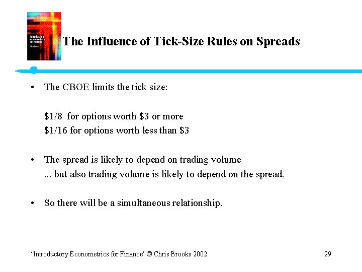
The Influence of Tick-Size Rules on Spreads • The CBOE limits the tick size: $1/8 for options worth $3 or more $1/16 for options worth less than $3 • The spread is likely to depend on trading volume. . . but also trading volume is likely to depend on the spread. • So there will be a simultaneous relationship. ‘Introductory Econometrics for Finance’ © Chris Brooks 2002 29

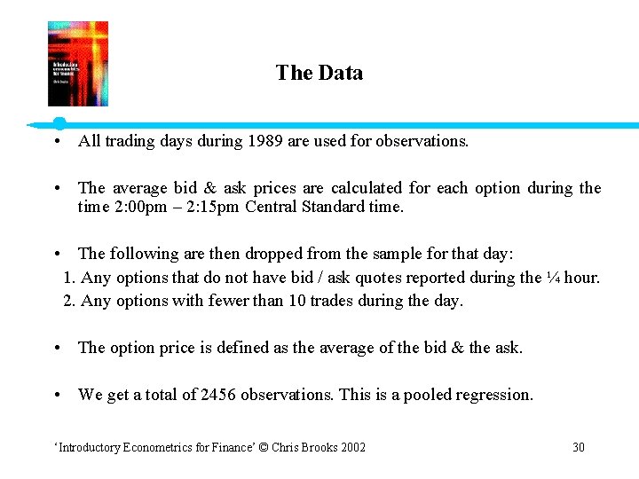
The Data • All trading days during 1989 are used for observations. • The average bid & ask prices are calculated for each option during the time 2: 00 pm – 2: 15 pm Central Standard time. • The following are then dropped from the sample for that day: 1. Any options that do not have bid / ask quotes reported during the ¼ hour. 2. Any options with fewer than 10 trades during the day. • The option price is defined as the average of the bid & the ask. • We get a total of 2456 observations. This is a pooled regression. ‘Introductory Econometrics for Finance’ © Chris Brooks 2002 30

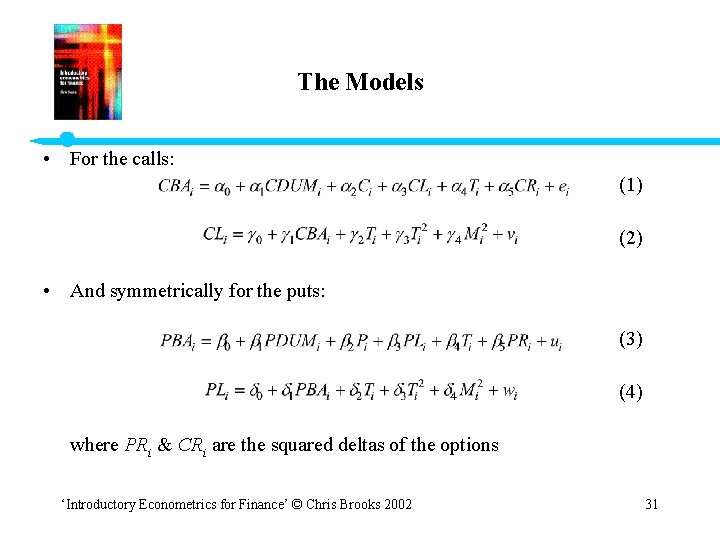
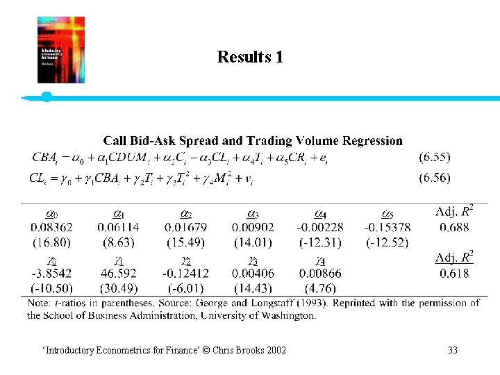
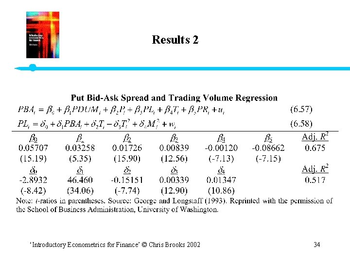
The Models • For the calls: (1) (2) • And symmetrically for the puts: (3) (4) where PRi & CRi are the squared deltas of the options ‘Introductory Econometrics for Finance’ © Chris Brooks 2002 31

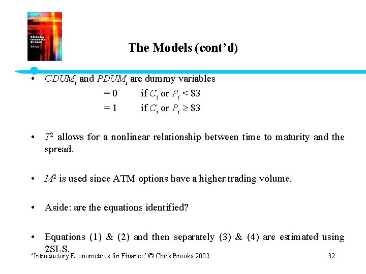
The Models (cont’d) • CDUMi and PDUMi are dummy variables = 0 if Ci or Pi < $3 = 1 if Ci or Pi $3 • T 2 allows for a nonlinear relationship between time to maturity and the spread. • M 2 is used since ATM options have a higher trading volume. • Aside: are the equations identified? • Equations (1) & (2) and then separately (3) & (4) are estimated using 2 SLS. ‘Introductory Econometrics for Finance’ © Chris Brooks 2002 32

Results 1 ‘Introductory Econometrics for Finance’ © Chris Brooks 2002 33

Results 2 ‘Introductory Econometrics for Finance’ © Chris Brooks 2002 34

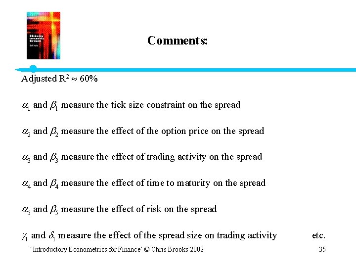
Comments: Adjusted R 2 60% 1 and 1 measure the tick size constraint on the spread 2 and 2 measure the effect of the option price on the spread 3 and 3 measure the effect of trading activity on the spread 4 and 4 measure the effect of time to maturity on the spread 5 and 5 measure the effect of risk on the spread 1 and 1 measure the effect of the spread size on trading activity etc. ‘Introductory Econometrics for Finance’ © Chris Brooks 2002 35

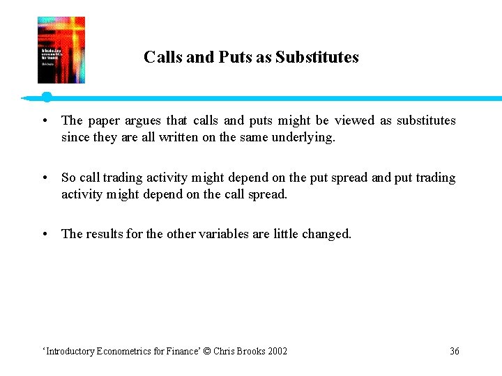
Calls and Puts as Substitutes • The paper argues that calls and puts might be viewed as substitutes since they are all written on the same underlying. • So call trading activity might depend on the put spread and put trading activity might depend on the call spread. • The results for the other variables are little changed. ‘Introductory Econometrics for Finance’ © Chris Brooks 2002 36

Conclusions • Bid - Ask spread variations between options can be explained by reference to the level of trading activity, deltas, time to maturity etc. There is a 2 way relationship between volume and the spread. • The authors argue that in the second part of the paper, they did indeed find evidence of substitutability between calls & puts. Comments - No diagnostics. - Why do the CL and PL equations not contain the CR and PR variables? - The authors could have tested for endogeneity of CBA and CL. - Why are the squared terms in maturity and moneyness only in the liquidity regressions? - Wrong sign on the squared deltas. ‘Introductory Econometrics for Finance’ © Chris Brooks 2002 37

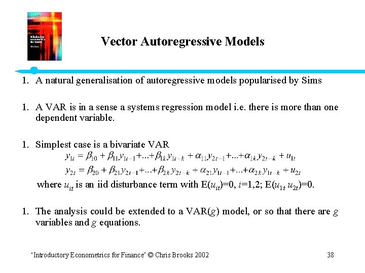
Vector Autoregressive Models 1. A natural generalisation of autoregressive models popularised by Sims 1. A VAR is in a sense a systems regression model i. e. there is more than one dependent variable. 1. Simplest case is a bivariate VAR where uit is an iid disturbance term with E(uit)=0, i=1, 2; E(u 1 t u 2 t)=0. 1. The analysis could be extended to a VAR(g) model, or so that there are g variables and g equations. ‘Introductory Econometrics for Finance’ © Chris Brooks 2002 38

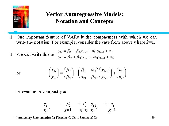
Vector Autoregressive Models: Notation and Concepts 1. One important feature of VARs is the compactness with which we can write the notation. For example, consider the case from above where k=1. 1. We can write this as or or even more compactly as yt = 0 + 1 yt-1 + ut g 1 g g g 1 ‘Introductory Econometrics for Finance’ © Chris Brooks 2002 39

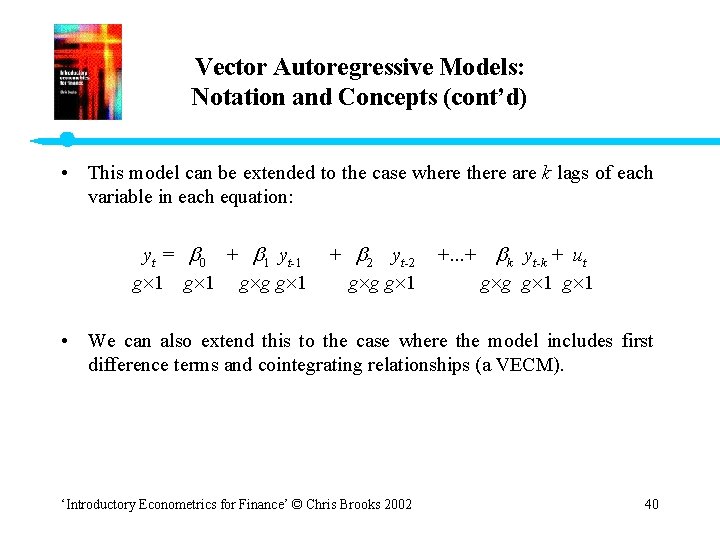
Vector Autoregressive Models: Notation and Concepts (cont’d) • This model can be extended to the case where there are k lags of each variable in each equation: yt = 0 + 1 yt-1 + 2 yt-2 +. . . + k yt-k + ut g 1 g g g 1 • We can also extend this to the case where the model includes first difference terms and cointegrating relationships (a VECM). ‘Introductory Econometrics for Finance’ © Chris Brooks 2002 40

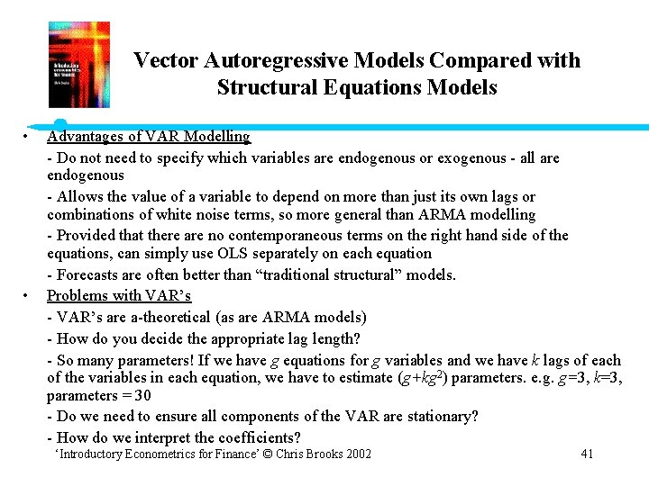
Vector Autoregressive Models Compared with Structural Equations Models • • Advantages of VAR Modelling - Do not need to specify which variables are endogenous or exogenous - all are endogenous - Allows the value of a variable to depend on more than just its own lags or combinations of white noise terms, so more general than ARMA modelling - Provided that there are no contemporaneous terms on the right hand side of the equations, can simply use OLS separately on each equation - Forecasts are often better than “traditional structural” models. Problems with VAR’s - VAR’s are a-theoretical (as are ARMA models) - How do you decide the appropriate lag length? - So many parameters! If we have g equations for g variables and we have k lags of each of the variables in each equation, we have to estimate (g+kg 2) parameters. e. g. g=3, k=3, parameters = 30 - Do we need to ensure all components of the VAR are stationary? - How do we interpret the coefficients? ‘Introductory Econometrics for Finance’ © Chris Brooks 2002 41

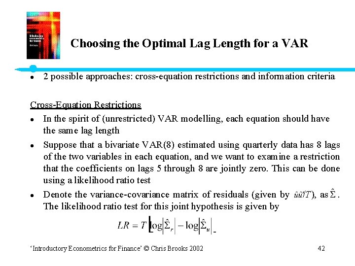
Choosing the Optimal Lag Length for a VAR 2 possible approaches: cross-equation restrictions and information criteria Cross-Equation Restrictions l In the spirit of (unrestricted) VAR modelling, each equation should have the same lag length l Suppose that a bivariate VAR(8) estimated using quarterly data has 8 lags of the two variables in each equation, and we want to examine a restriction that the coefficients on lags 5 through 8 are jointly zero. This can be done using a likelihood ratio test l Denote the variance-covariance matrix of residuals (given by /T), as . The likelihood ratio test for this joint hypothesis is given by l ‘Introductory Econometrics for Finance’ © Chris Brooks 2002 42

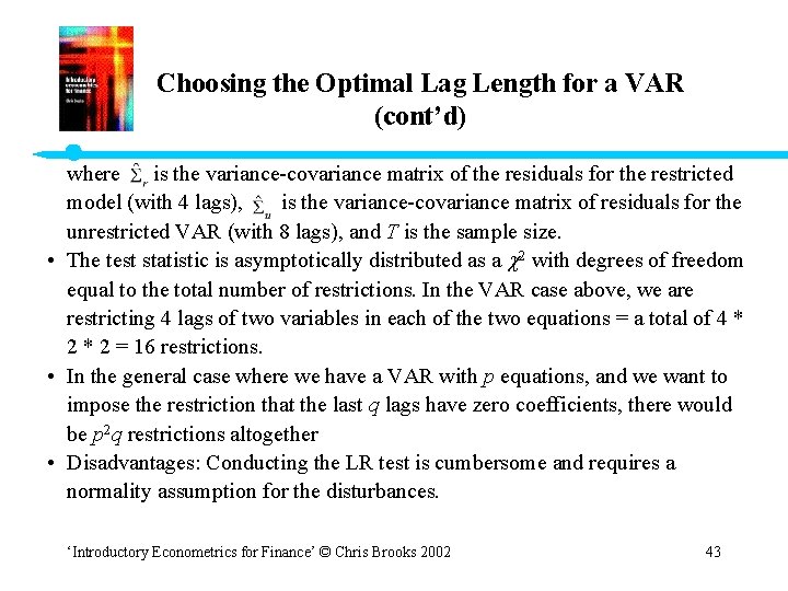
Choosing the Optimal Lag Length for a VAR (cont’d) where is the variance-covariance matrix of the residuals for the restricted model (with 4 lags), is the variance-covariance matrix of residuals for the unrestricted VAR (with 8 lags), and T is the sample size. • The test statistic is asymptotically distributed as a 2 with degrees of freedom equal to the total number of restrictions. In the VAR case above, we are restricting 4 lags of two variables in each of the two equations = a total of 4 * 2 = 16 restrictions. • In the general case where we have a VAR with p equations, and we want to impose the restriction that the last q lags have zero coefficients, there would be p 2 q restrictions altogether • Disadvantages: Conducting the LR test is cumbersome and requires a normality assumption for the disturbances. ‘Introductory Econometrics for Finance’ © Chris Brooks 2002 43

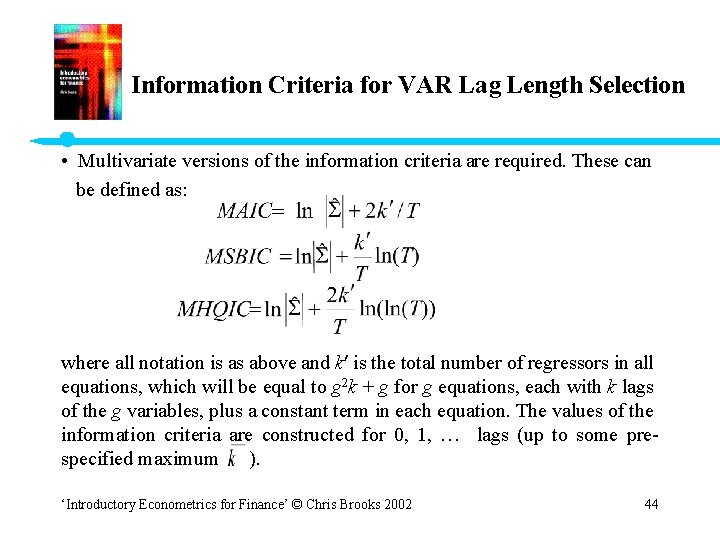
Information Criteria for VAR Lag Length Selection • Multivariate versions of the information criteria are required. These can be defined as: where all notation is as above and k is the total number of regressors in all equations, which will be equal to g 2 k + g for g equations, each with k lags of the g variables, plus a constant term in each equation. The values of the information criteria are constructed for 0, 1, … lags (up to some prespecified maximum ). ‘Introductory Econometrics for Finance’ © Chris Brooks 2002 44

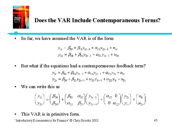
Does the VAR Include Contemporaneous Terms? • So far, we have assumed the VAR is of the form • But what if the equations had a contemporaneous feedback term? • We can write this as • This VAR is in primitive form. ‘Introductory Econometrics for Finance’ © Chris Brooks 2002 45

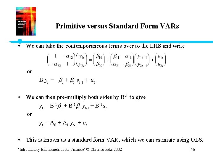
Primitive versus Standard Form VARs • We can take the contemporaneous terms over to the LHS and write or B yt = 0 + 1 yt-1 + ut • We can then pre-multiply both sides by B-1 to give yt = B-1 0 + B-1 1 yt-1 + B-1 ut or yt = A 0 + A 1 yt-1 + et • This is known as a standard form VAR, which we can estimate using OLS. ‘Introductory Econometrics for Finance’ © Chris Brooks 2002 46

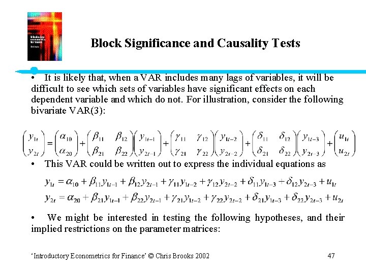
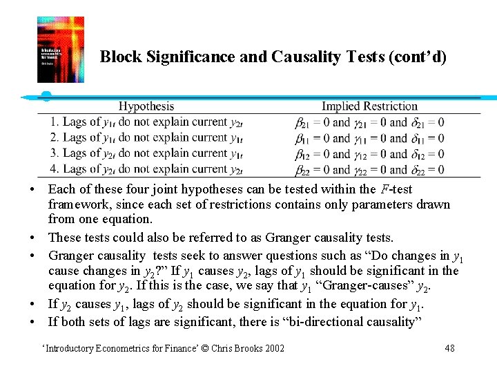
Block Significance and Causality Tests • It is likely that, when a VAR includes many lags of variables, it will be difficult to see which sets of variables have significant effects on each dependent variable and which do not. For illustration, consider the following bivariate VAR(3): • This VAR could be written out to express the individual equations as • We might be interested in testing the following hypotheses, and their implied restrictions on the parameter matrices: ‘Introductory Econometrics for Finance’ © Chris Brooks 2002 47

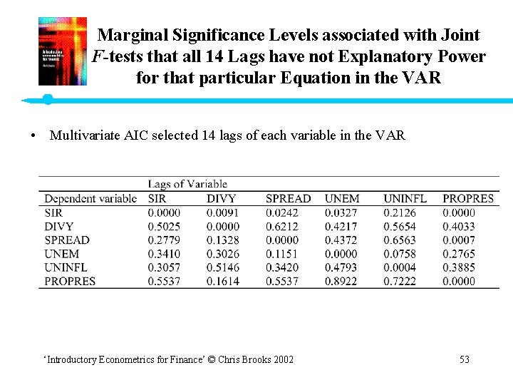
Block Significance and Causality Tests (cont’d) • Each of these four joint hypotheses can be tested within the F-test framework, since each set of restrictions contains only parameters drawn from one equation. • These tests could also be referred to as Granger causality tests. • Granger causality tests seek to answer questions such as “Do changes in y 1 cause changes in y 2? ” If y 1 causes y 2, lags of y 1 should be significant in the equation for y 2. If this is the case, we say that y 1 “Granger-causes” y 2. • If y 2 causes y 1, lags of y 2 should be significant in the equation for y 1. • If both sets of lags are significant, there is “bi-directional causality” ‘Introductory Econometrics for Finance’ © Chris Brooks 2002 48

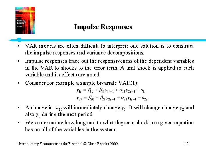
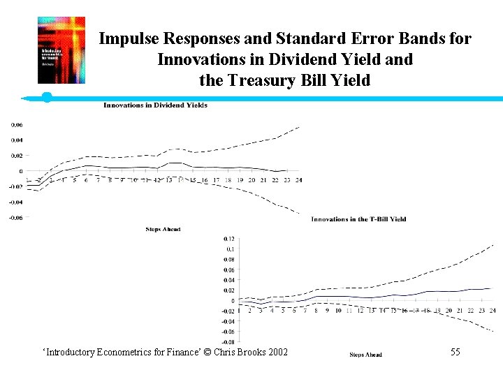
Impulse Responses • VAR models are often difficult to interpret: one solution is to construct the impulse responses and variance decompositions. • Impulse responses trace out the responsiveness of the dependent variables in the VAR to shocks to the error term. A unit shock is applied to each variable and its effects are noted. • Consider for example a simple bivariate VAR(1): • A change in u 1 t will immediately change y 1. It will change y 2 and also y 1 during the next period. • We can examine how long and to what degree a shock to a given equation has on all of the variables in the system. ‘Introductory Econometrics for Finance’ © Chris Brooks 2002 49

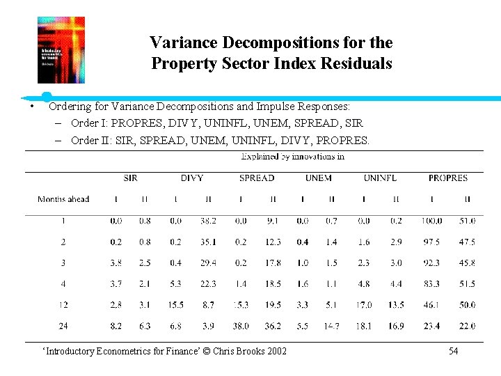
Variance Decompositions • Variance decompositions offer a slightly different method of examining VAR dynamics. They give the proportion of the movements in the dependent variables that are due to their “own” shocks, versus shocks to the other variables. • This is done by determining how much of the s-step ahead forecast error variance for each variable is explained innovations to each explanatory variable (s = 1, 2, …). • The variance decomposition gives information about the relative importance of each shock to the variables in the VAR. ‘Introductory Econometrics for Finance’ © Chris Brooks 2002 50

Impulse Responses and Variance Decompositions: The Ordering of the Variables • But for calculating impulse responses and variance decompositions, the ordering of the variables is important. • The main reason for this is that above, we assumed that the VAR error terms were statistically independent of one another. • This is generally not true, however. The error terms will typically be correlated to some degree. • Therefore, the notion of examining the effect of the innovations separately has little meaning, since they have a common component. • What is done is to “orthogonalise” the innovations. • In the bivariate VAR, this problem would be approached by attributing all of the effect of the common component to the first of the two variables in the VAR. • In the general case where there are more variables, the situation is more complex but the interpretation is the same. ‘Introductory Econometrics for Finance’ © Chris Brooks 2002 51

An Example of the use of VAR Models: The Interaction between Property Returns and the Macroeconomy. • • Brooks and Tsolacos (1999) employ a VAR methodology for investigating the interaction between the UK property market and various macroeconomic variables. Monthly data are used for the period December 1985 to January 1998. It is assumed that stock returns are related to macroeconomic and business conditions. The variables included in the VAR are – FTSE Property Total Return Index (with general stock market effects removed) – The rate of unemployment – Nominal interest rates – The spread between long and short term interest rates – Unanticipated inflation – The dividend yield. The property index and unemployment are I(1) and hence are differenced. ‘Introductory Econometrics for Finance’ © Chris Brooks 2002 52

Marginal Significance Levels associated with Joint F-tests that all 14 Lags have not Explanatory Power for that particular Equation in the VAR • Multivariate AIC selected 14 lags of each variable in the VAR ‘Introductory Econometrics for Finance’ © Chris Brooks 2002 53

Variance Decompositions for the Property Sector Index Residuals • Ordering for Variance Decompositions and Impulse Responses: – Order I: PROPRES, DIVY, UNINFL, UNEM, SPREAD, SIR – Order II: SIR, SPREAD, UNEM, UNINFL, DIVY, PROPRES. ‘Introductory Econometrics for Finance’ © Chris Brooks 2002 54

Impulse Responses and Standard Error Bands for Innovations in Dividend Yield and the Treasury Bill Yield ‘Introductory Econometrics for Finance’ © Chris Brooks 2002 55