Applied Econometrics using MATLAB Chapter 4 Regression Diagnostics

Applied Econometrics using MATLAB Chapter 4 Regression Diagnostics 資管所 黃立文

Introduction • The first section of this chapter introduces functions for diagnosing and correcting collinearity problems. • The last section discusses functions to detect and correct for outliers and influential observations in regression problems.

Collinearity diagnostics and procedures • Collinearity problem is that near linear relations among the explanatory variable vectors tends to degrade the precision of the estimated parameters.

Collinearity diagnostics and procedures • One way to illustrate the increase in dispersion of the least-squares estimates is with a Monte Carlo experiment. – generate a set of y vectors from a model where the explanatory variables are reasonably orthogonal, involving no near linear dependencies. – Alternative sets of y vectors are then generated from a model where the explanatory variables become increasingly collinear.

Collinearity diagnostics and procedures • The specific experiment involved using three explanatory variables in a model shown in :

Collinearity diagnostics and procedures •

Collinearity diagnostics and procedures • To create collinear relations we used the scheme shown in (4. 2) where we no longer generate the X 2 and X 3 vectors independently. • Instead, we generate the X 2 vector from the X 3 vector with an added random error vector u.

Collinearity diagnostics and procedures •

Collinearity diagnostics and procedures – Two additional sets of 1000 Y vectors were generated in the same manner based on the same X 3 and X 1 vectors, but with two new versions of the X 2 vector generated from X 3. The new X 2 vectors were produced by decreasing the variance of the random vector u to 0. 5 and 0. 1, respectively.

Collinearity diagnostics and procedures • The MATLAB code to produce this experiment is:

Collinearity diagnostics and procedures • The results of the experiment showing both the means and standard deviations from the distribution of estimates are:

Collinearity diagnostics and procedures •

Function bkw() Belsley, Kuh, and Welsch (1980) • The diagnostic is capable of determining the number of near linear dependencies in a given data matrix X, and the diagnostic identifies which variables are involved in each linear dependency.

Function bkw() •

Function bkw() •

Function bkw() •

Function bkw() It is shown in Belsley, Kuh and Welsch (1980) that a large value of the condition index, is associated with each near linear dependency, and the variates involved in the dependency are those with large proportions of their variance associated with large magnitudes.

Function bkw() • Belsley, Kuh, and Welsch (1980) determined that variance-decomposition proportions in excess of 0. 5 indicate the variates involved in specific linear dependencies. The joint condition of magnitudes for

Function bkw() • An example of BKW:

Function bkw()

Function bkw() The results of the program are shown below. They detect the near linear relationship between variables 1, 2 and 4 which we generated in the data matrix X.

Function ridge() •

Function ridge() •

Function ridge() •

Function ridge() •

Function ridge() •

Function ridge() • As an example, consider the following MATLAB program

Function ridge() • Result:

Function ridge() •

Function rtrace • A function rtrace helps to assess the trade-off between bias and efficiency by plotting the ridge estimates for a range of alternative values of the ridge parameter. The documentation for rtrace is:

Function rtrace • As an example of using this function

Function rtrace

Outlier diagnostics and procedures • Outlier observations are known to adversely impact least-squares estimates because the aberrant observations generate large errors. • Function dfbeta produces a set of diagnostics discussed in Belsley, Kuh and Welsch (1980).

Function dfbeta • The function dfbeta returns a structure that can be used to produce graphical output.

Function dfbeta •

Function dfbeta

Outlier diagnostics and procedures • A number of alternative estimation methods exist that attempt to downweight outliers. The regression library contains a function robust and olst as well as lad that we developed in Chapter 3. The documentation for robust is:

Function robust

Function robust • An example:

Function olst • The routine olst performs regression based on an assumption that the errors are t-distributed rather than normal, which allows for “fattailed“ error distributions. The documentation is: T-distribution PDF

Function olst

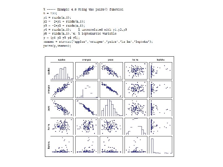
Function pair • Another graphical tool for regression diagnostics is the pairs function that produces pairwise scatterplots for a group of variables as well as histograms of the distribution of observations for each variable.