Econometrics Chengyuan Yin School of Mathematics Applied Econometrics

Econometrics Chengyuan Yin School of Mathematics

Applied Econometrics 7. Estimating the Variance of the Least Squares Estimator

Context The true variance of b is 2 E[(X X)-1] We consider how to use the sample data to estimate this matrix. The ultimate objectives are to form interval estimates for regression slopes and to test hypotheses about them. Both require estimates of the variability of the distribution. We then examine a factor which affects how "large" this variance is, multicollinearity.

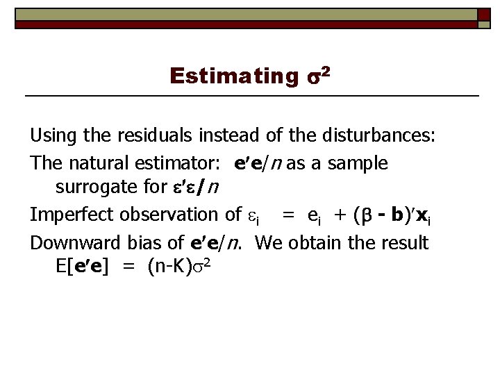
Estimating 2 Using the residuals instead of the disturbances: The natural estimator: e e/n as a sample surrogate for /n Imperfect observation of i = ei + ( - b) xi Downward bias of e e/n. We obtain the result E[e e] = (n-K) 2

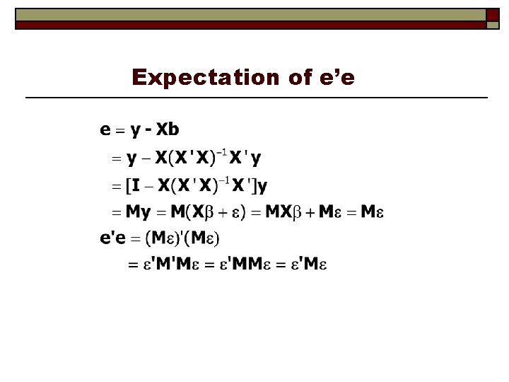
Expectation of e’e

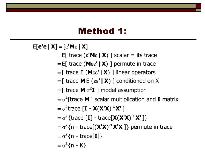
Method 1:

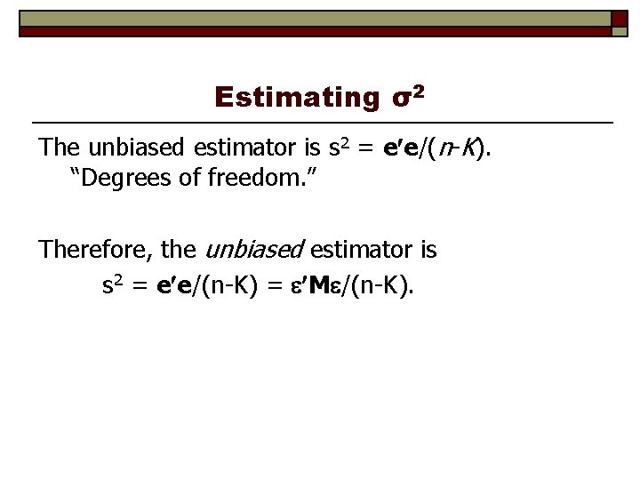
Estimating σ2 The unbiased estimator is s 2 = e e/(n-K). “Degrees of freedom. ” Therefore, the unbiased estimator is s 2 = e e/(n-K) = M /(n-K).

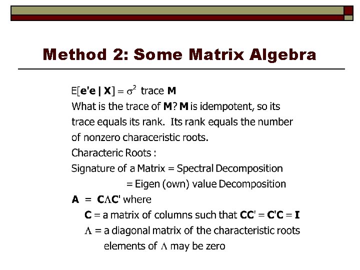
Method 2: Some Matrix Algebra

Decomposing M

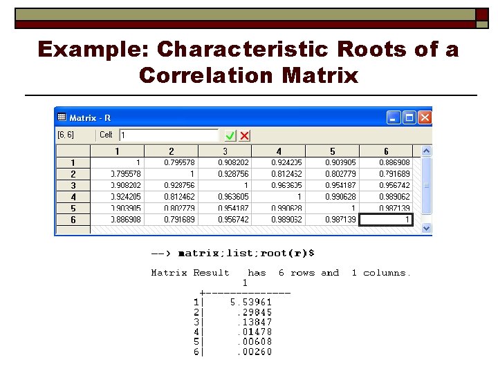
Example: Characteristic Roots of a Correlation Matrix

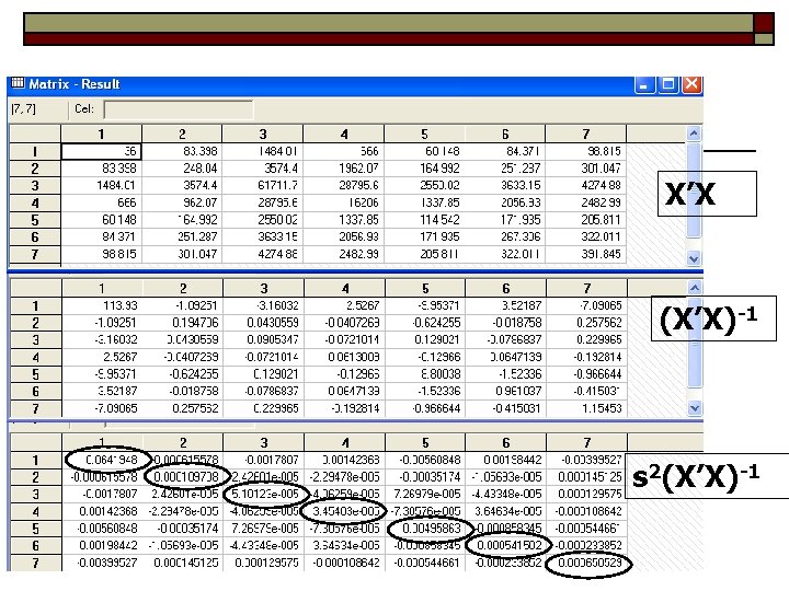
Var[b|X] Estimating the Covariance Matrix for b|X The true covariance matrix is 2 (X’X)-1 The natural estimator is s 2(X’X)-1 “Standard errors” of the individual coefficients. How does the conditional variance 2(X’X)-1 differ from the unconditional one, 2 E[(X’X)-1]?

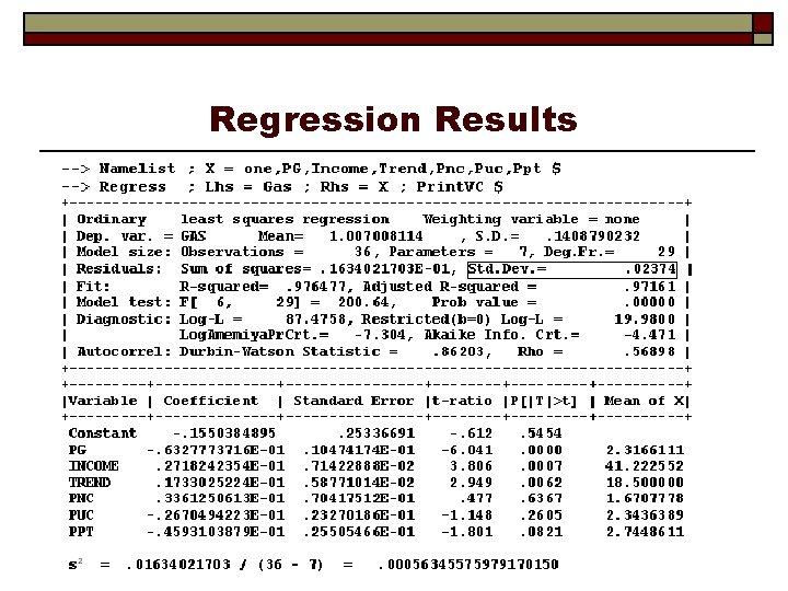
Regression Results

X’X (X’X)-1 s 2(X’X)-1

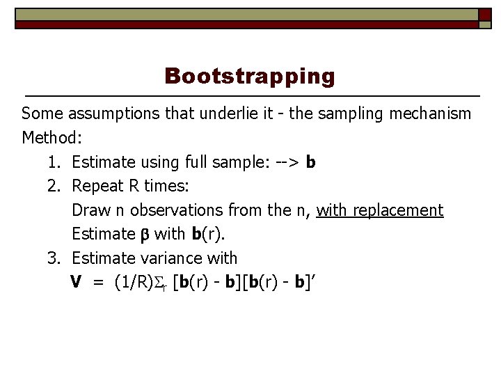
Bootstrapping Some assumptions that underlie it - the sampling mechanism Method: 1. Estimate using full sample: --> b 2. Repeat R times: Draw n observations from the n, with replacement Estimate with b(r). 3. Estimate variance with V = (1/R) r [b(r) - b]’

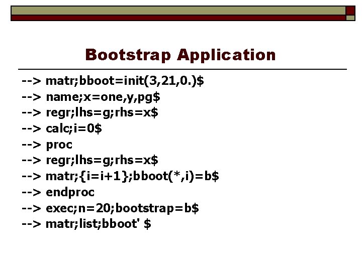
Bootstrap Application --> matr; bboot=init(3, 21, 0. )$ --> name; x=one, y, pg$ --> regr; lhs=g; rhs=x$ --> calc; i=0$ --> proc --> regr; lhs=g; rhs=x$ --> matr; {i=i+1}; bboot(*, i)=b$ --> endproc --> exec; n=20; bootstrap=b$ --> matr; list; bboot' $

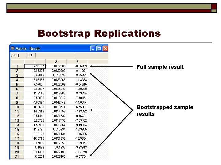
+--------------+--------+--------+-----+ |Variable| Coefficient | Standard Error |t-ratio |P[|T|>t]| Mean of X| +--------------+--------+--------+-----+ Constant| 7. 96106957 6. 23310198 1. 277. 2104 Y |. 01226831. 00094696 12. 955. 0000 9232. 86111 PG | -8. 86289207 1. 35142882 -6. 558. 0000 2. 31661111 Completed 20 bootstrap iterations. +---------------------+ | Results of bootstrap estimation of model. | | Model has been reestimated 20 times. | | Means shown below are the means of the | | bootstrap estimates. Coefficients shown | | below are the original estimates based | | on the full sample. | | bootstrap samples have 36 observations. | +---------------------+ +--------------+--------+--------+-----+ |Variable| Coefficient | Standard Error |b/St. Er. |P[|Z|>z]| Mean of X| +--------------+--------+--------+-----+ B 001 | 7. 96106957 6. 72472102 1. 184. 2365 4. 22761200 B 002 |. 01226831. 00112983 10. 859. 0000. 01285738 B 003 | -8. 86289207 1. 94703780 -4. 552. 0000 -9. 45989851

Bootstrap Replications Full sample result Bootstrapped sample results

Multicollinearity Not “short rank, ” which is a deficiency in the model. A characteristic of the data set which affects the covariance matrix. Regardless, is unbiased. Consider one of the unbiased coefficient estimators of k. E[bk] = k Var[b] = 2(X’X)-1. The variance of bk is the kth diagonal element of 2(X’X)-1. We can isolate this with the result in your text. Let [ [X, z] be [Other xs, xk] = [X 1, x 2] (a convenient notation for the results in the text). We need the residual maker, M 1. The general result is that the diagonal element we seek is [x 2 M 1 x 2]-1 , which we know is the reciprocal of the sum of squared residuals in the regression of x 2 on X 1. The remainder of the derivation of the result we seek is in your text. The estimated variance of bk is

Variance of a Least Squares Coefficient Estimator Estimated Var[bk] =

Multicollinearity Clearly, the greater the fit of the regression in the regression of x 2 on X 1, the greater is the variance. In the limit, a perfect fit produces an infinite variance. There is no “cure” for collinearity. Estimating something else is not helpful (principal components, for example). There are “measures” of multicollinearity, such as the condition number of X. Best approach: Be cognizant of it. Understand its implications for estimation. A familiar application: The Longley data. See data table F 4. 2 Very prevalent in macroeconomic data, especially low frequency (e. g. , yearly). Made worse by taking logs. What is better: Include a variable that causes collinearity, or drop the variable and suffer from a biased estimator? Mean squared error would be the basis for comparison. Some generalities.