CHAPTER 12 AUTOCORRELATION WHAT HAPPENS IF THE ERROR

CHAPTER 12. AUTOCORRELATION: WHAT HAPPENS IF THE ERROR TERMS ARE CORRELATED?

Questions in Autocorrelation: n The nature of autocorrelation? n The theoretical and practical consequences of autocorrelation? n Detection of autocorrelation? n Remedies of autocorrelation?

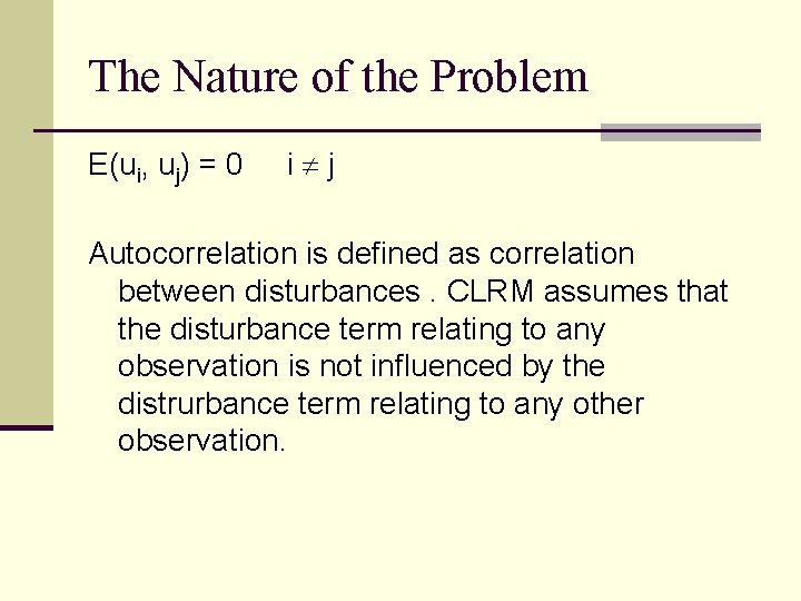
The Nature of the Problem E(ui, uj) = 0 i j Autocorrelation is defined as correlation between disturbances. CLRM assumes that the disturbance term relating to any observation is not influenced by the distrurbance term relating to any other observation.

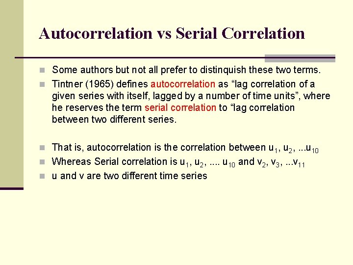
Autocorrelation vs Serial Correlation n Some authors but not all prefer to distinquish these two terms. n Tintner (1965) defines autocorrelation as “lag correlation of a given series with itself, lagged by a number of time units”, where he reserves the term serial correlation to “lag correlation between two different series. n That is, autocorrelation is the correlation between u 1, u 2, . . . u 10 n Whereas Serial correlation is u 1, u 2, . . u 10 and v 2, v 3, . . . v 11 n u and v are two different time series

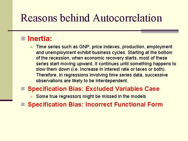
Reasons behind Autocorrelation n Inertia: n Time series such as GNP, price indexes, production, employment and unemployment exhibit business cycles. Starting at the bottom of the recession, when economic recovery starts, most of these series start moving upward. It continues until something happens to slow them down (i. e. Increase in interest rate or taxes or both). Therefore, in regressions involving time series data, successive observations are likely to be interdependent. n Specification Bias: Excluded Variables Case n Some true regressors might be missed in the models n Specification Bias: Incorrect Functional Form

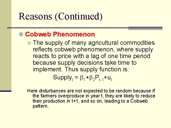
Reasons (Continued) n Cobweb Phenomenon n The supply of many agricultural commodities reflects cobweb phenomenon, where supply reacts to price with a lag of one time period because supply decisions take time to implement. Thus supply function is: Supplyt = 1+ 2 Pt-1+ut Here disturbances are not expected to be random because if the farmers overproduce in year t, they are likely to reduce their production in t+1, and so on, leading to a Cobweb pattern.

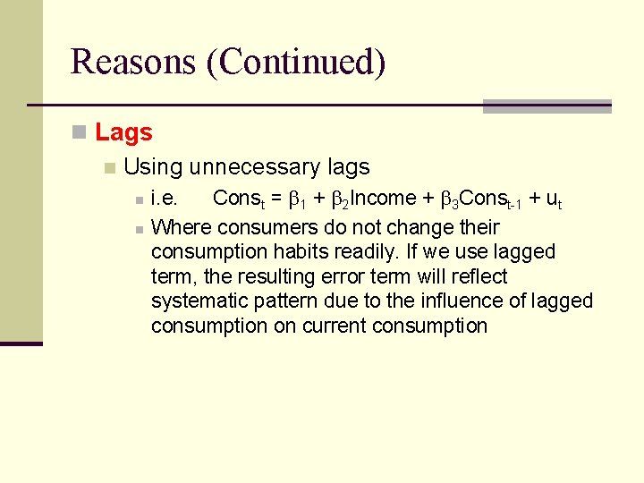
Reasons (Continued) n Lags n Using unnecessary lags n n i. e. Const = 1 + 2 Income + 3 Const-1 + ut Where consumers do not change their consumption habits readily. If we use lagged term, the resulting error term will reflect systematic pattern due to the influence of lagged consumption on current consumption

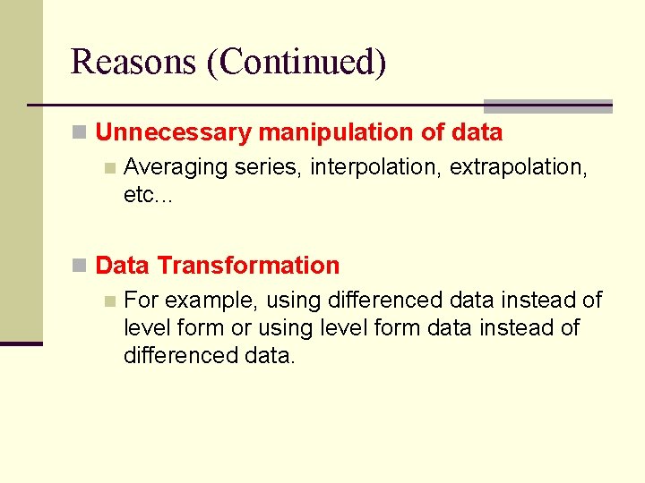
Reasons (Continued) n Unnecessary manipulation of data n Averaging series, interpolation, extrapolation, etc. . . n Data Transformation n For example, using differenced data instead of level form or using level form data instead of differenced data.

Reasons (Continued) n Non – Stationarity (Chapter 21) n A time series is stationary if its characteristics (mean, variance, covariance) are time variant; that is, they do not change over time. Nonstationarity may cause autocorrelation.

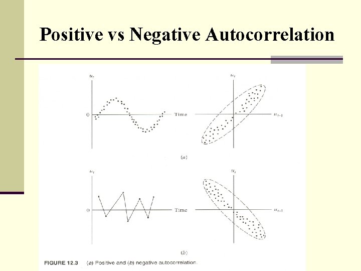
Positive vs Negative Autocorrelation

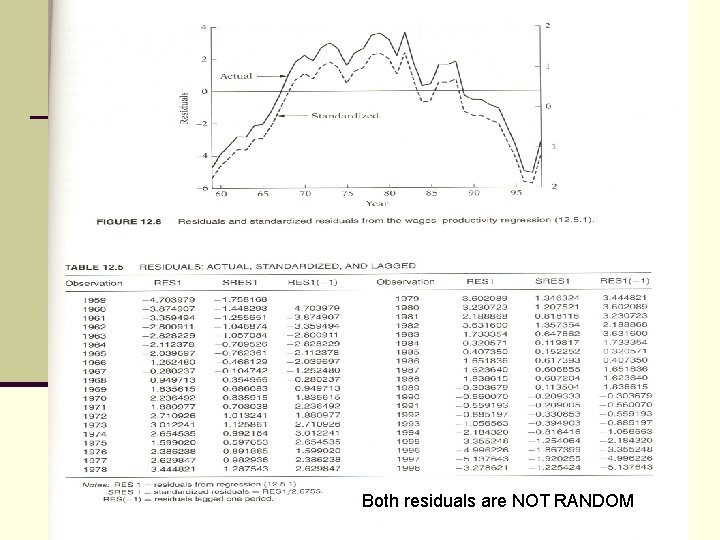
Detecting Autocorrelation -1 n Plotting residuals and standardized residuals of regression against time and compare if they show similar pattern which signs for autocorrelation n Standardized residuals= residuals / st. error of regression.

Both residuals are NOT RANDOM

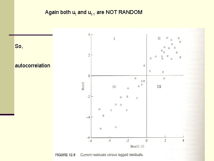
Again both ut and ut-1 are NOT RANDOM So, autocorrelation

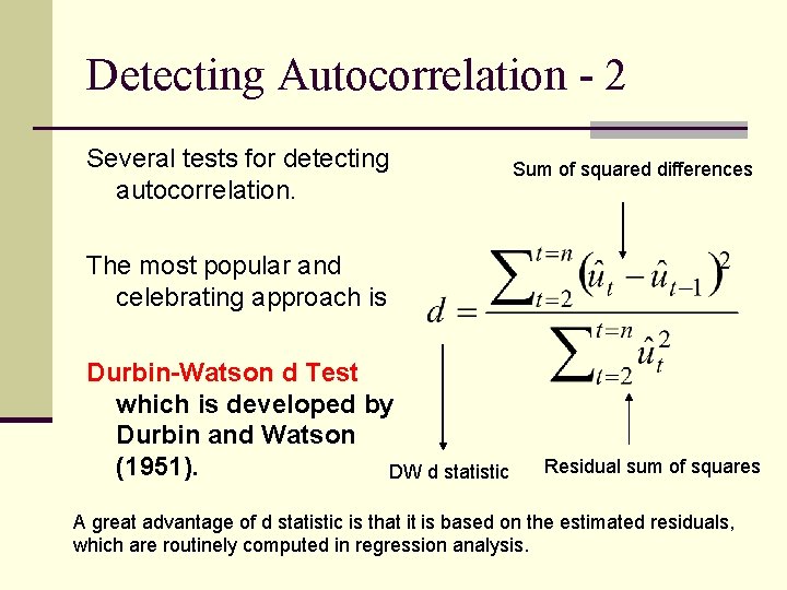
Detecting Autocorrelation - 2 Several tests for detecting autocorrelation. Sum of squared differences The most popular and celebrating approach is Durbin-Watson d Test which is developed by Durbin and Watson (1951). DW d statistic Residual sum of squares A great advantage of d statistic is that it is based on the estimated residuals, which are routinely computed in regression analysis.

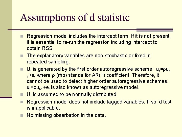
Assumptions of d statistic n Regression model includes the intercept term. If it is not present, n n n it is essential to re-run the regression including intercept to obtain RSS. The explanatory variables are non-stochastic or fixed in repeated sampling. Ut is generated by the first order autoregressive scheme: ut=ρut 1+et where ρ (rho) stands for AR(1) coefficient. Therefore, it cannot be used to detect higher order autoregressive schemes. ut=ρut-1+et is also known as autoregressive model. Ut is assumed to be normally distributed. Regression model does not include lagged variables. If so, d test is inapplicable. No missing obserbation in the data.

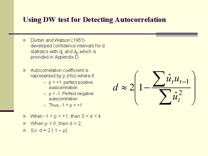
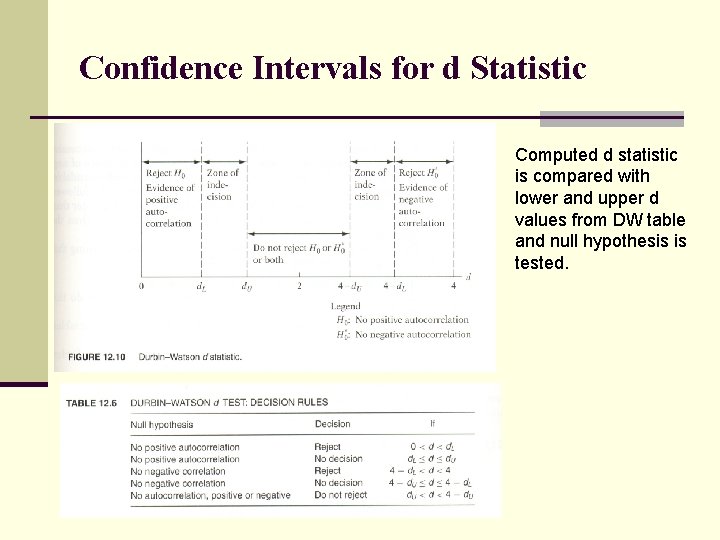
Using DW test for Detecting Autocorrelation n Durbin and Watson (1951) developed confidence intervals for d statistics with d. L and d. U which is provided in Appendix D. n Autocorrelation coefficient is represented by ρ (rho) where if: n n ρ = +1: perfect positive autocorrelation ρ = -1: Perfect negative autocorrelation Thus, -1 < ρ < +1 When -1 < ρ < +1, then 0 < d < 4 n When ρ = 0, then d = 2, n So: d ≈ 2 ( 1 – ρ)

Confidence Intervals for d Statistic Computed d statistic is compared with lower and upper d values from DW table and null hypothesis is tested.

APPLICATION TO MONEY AND INCOME DATA FOR JAPAN