Error and Error Analysis Types of error Random

Error and Error Analysis

Types of error Random error – Unbiased error due to unpredictable fluctuations in the environment, measuring device, and so forth. Systematic error – Error that biases a result in a particular direction. This can be due to calibration error, instrumental bias, errors in the approximations used in the data analysis, and so forth. For example, if we carried out several independent measurements of the normal boiling point of a pure unknown liquid, we would expect some scatter in the data due to random differences that occur from measurement to measurement. If thermometer used in the measurements was not calibrated, or we failed to correct the measurements for the effect of pressure on boiling point, there would be systematic errors.

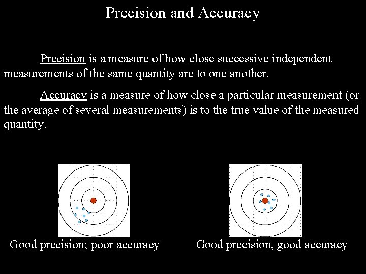
Precision and Accuracy Precision is a measure of how close successive independent measurements of the same quantity are to one another. Accuracy is a measure of how close a particular measurement (or the average of several measurements) is to the true value of the measured quantity. Good precision; poor accuracy Good precision, good accuracy

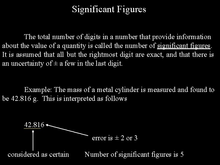
Significant Figures The total number of digits in a number that provide information about the value of a quantity is called the number of significant figures. It is assumed that all but the rightmost digit are exact, and that there is an uncertainty of ± a few in the last digit. Example: The mass of a metal cylinder is measured and found to be 42. 816 g. This is interpreted as follows 42. 816 error is ± 2 or 3 considered as certain Number of significant figures is 5

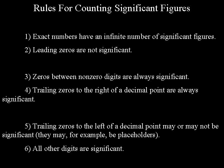
Rules For Counting Significant Figures 1) Exact numbers have an infinite number of significant figures. 2) Leading zeros are not significant. 3) Zeros between nonzero digits are always significant. 4) Trailing zeros to the right of a decimal point are always significant. 5) Trailing zeros to the left of a decimal point may or may not be significant (they may, for example, be placeholders). 6) All other digits are significant.

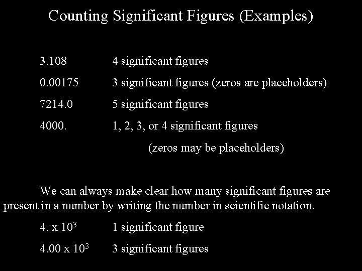
Counting Significant Figures (Examples) 3. 108 4 significant figures 0. 00175 3 significant figures (zeros are placeholders) 7214. 0 5 significant figures 4000. 1, 2, 3, or 4 significant figures (zeros may be placeholders) We can always make clear how many significant figures are present in a number by writing the number in scientific notation. 4. x 103 1 significant figure 4. 00 x 103 3 significant figures

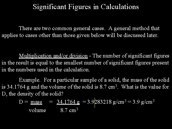
Significant Figures in Calculations There are two common general cases. A general method that applies to cases other than those given below will be discussed later. Multiplication and/or division - The number of significant figures in the result is equal to the smallest number of significant figures present in the numbers used in the calculation. Example. For a particular sample of a solid, the mass of the solid is 34. 1764 g and the volume of the solid is 8. 7 cm 3. What is the value for D, the density of the solid? D = mass = 34. 1764 g = 3. 9283218 g/cm 3 = 3. 9 g/cm 3 volume 8. 7 cm 3

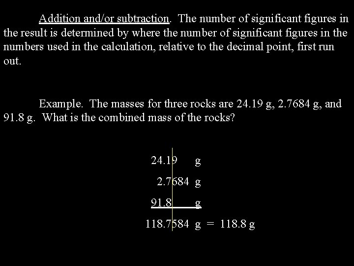
Addition and/or subtraction. The number of significant figures in the result is determined by where the number of significant figures in the numbers used in the calculation, relative to the decimal point, first run out. Example. The masses for three rocks are 24. 19 g, 2. 7684 g, and 91. 8 g. What is the combined mass of the rocks? 24. 19 g 2. 7684 g 91. 8 g 118. 7584 g = 118. 8 g

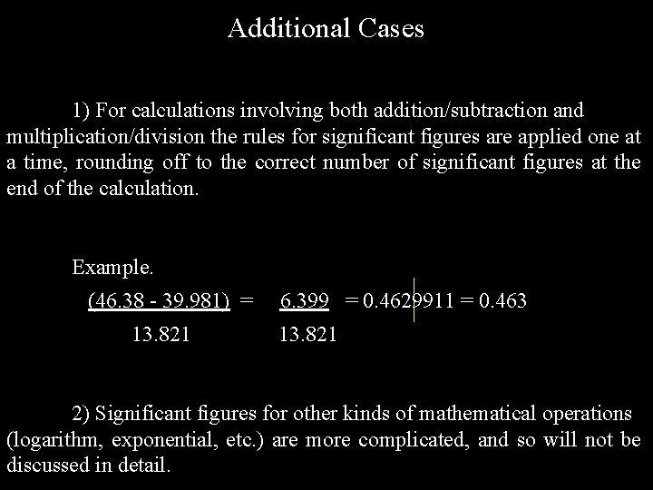
Additional Cases 1) For calculations involving both addition/subtraction and multiplication/division the rules for significant figures are applied one at a time, rounding off to the correct number of significant figures at the end of the calculation. Example. (46. 38 - 39. 981) = 13. 821 6. 399 = 0. 4629911 = 0. 463 13. 821 2) Significant figures for other kinds of mathematical operations (logarithm, exponential, etc. ) are more complicated, and so will not be discussed in detail.

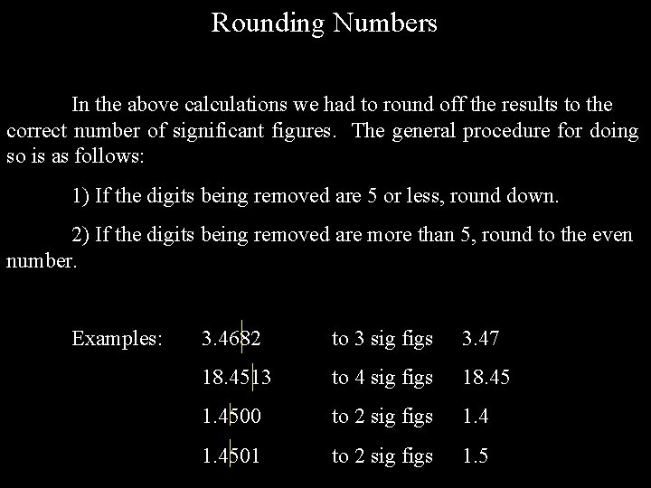
Rounding Numbers In the above calculations we had to round off the results to the correct number of significant figures. The general procedure for doing so is as follows: 1) If the digits being removed are 5 or less, round down. 2) If the digits being removed are more than 5, round to the even number. Examples: 3. 4682 to 3 sig figs 3. 47 18. 4513 to 4 sig figs 18. 45 1. 4500 to 2 sig figs 1. 4501 to 2 sig figs 1. 5

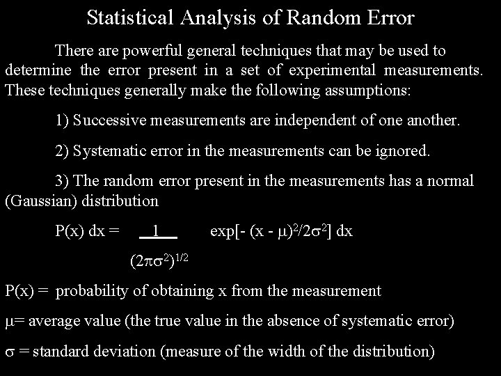
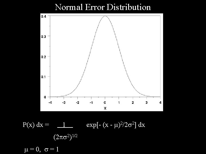
Statistical Analysis of Random Error There are powerful general techniques that may be used to determine the error present in a set of experimental measurements. These techniques generally make the following assumptions: 1) Successive measurements are independent of one another. 2) Systematic error in the measurements can be ignored. 3) The random error present in the measurements has a normal (Gaussian) distribution P(x) dx = 1 exp[- (x - )2/2 2] dx (2 2)1/2 P(x) = probability of obtaining x from the measurement = average value (the true value in the absence of systematic error) = standard deviation (measure of the width of the distribution)

Normal Error Distribution P(x) dx = 1 (2 2)1/2 = 0, = 1 exp[- (x - )2/2 2] dx

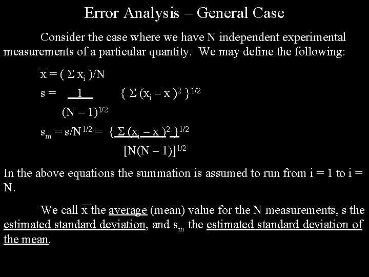
Error Analysis – General Case Consider the case where we have N independent experimental measurements of a particular quantity. We may define the following: x = ( xi )/N s= 1 { (xi – x )2 }1/2 (N – 1)1/2 sm = s/N 1/2 = { (xi – x )2 }1/2 [N(N – 1)]1/2 In the above equations the summation is assumed to run from i = 1 to i = N. We call x the average (mean) value for the N measurements, s the estimated standard deviation, and sm the estimated standard deviation of the mean.

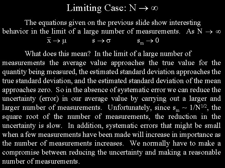
Limiting Case: N The equations given on the previous slide show interesting behavior in the limit of a large number of measurements. As N x s sm 0 What does this mean? In the limit of a large number of measurements the average value approaches the true value for the quantity being measured, the estimated standard deviation approaches the true standard deviation, and the estimated standard deviation of the mean approaches zero. So in the absence of systematic error we can reduce the uncertainty (error) in our average value by carrying out a larger and larger number of measurements. Unfortunately, since sm ~ 1/N 1/2, the square root of the number of measurements, the reduction in the uncertainty is slow. In addition, systematic errors that might be small when a few measurements have been made will increase in importance as the number of measurements increases. We normally have to make a compromise between reducing the uncertainty and making a reasonable number of measurements.

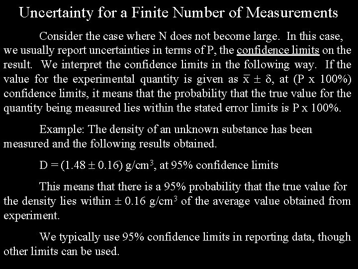
Uncertainty for a Finite Number of Measurements Consider the case where N does not become large. In this case, we usually report uncertainties in terms of P, the confidence limits on the result. We interpret the confidence limits in the following way. If the value for the experimental quantity is given as x , at (P x 100%) confidence limits, it means that the probability that the true value for the quantity being measured lies within the stated error limits is P x 100%. Example: The density of an unknown substance has been measured and the following results obtained. D = (1. 48 0. 16) g/cm 3, at 95% confidence limits This means that there is a 95% probability that the true value for the density lies within 0. 16 g/cm 3 of the average value obtained from experiment. We typically use 95% confidence limits in reporting data, though other limits can be used.

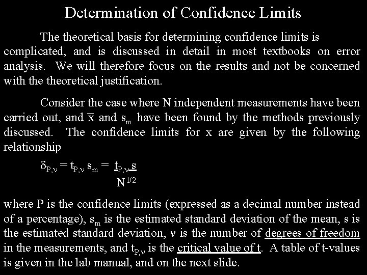
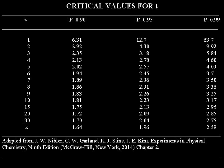
Determination of Confidence Limits The theoretical basis for determining confidence limits is complicated, and is discussed in detail in most textbooks on error analysis. We will therefore focus on the results and not be concerned with theoretical justification. Consider the case where N independent measurements have been carried out, and x and sm have been found by the methods previously discussed. The confidence limits for x are given by the following relationship P, = t. P, sm = t. P, s N 1/2 where P is the confidence limits (expressed as a decimal number instead of a percentage), sm is the estimated standard deviation of the mean, s is the estimated standard deviation, is the number of degrees of freedom in the measurements, and t. P, is the critical value of t. A table of t-values is given in the lab manual, and on the next slide.

CRITICAL VALUES FOR t ____________________________________________ P=0. 90 P=0. 95 P=0. 99 _______________________________________ 1 6. 31 12. 7 63. 7 2 2. 92 4. 30 9. 92 3 2. 35 3. 18 5. 84 4 2. 13 2. 78 4. 60 5 2. 02 2. 57 4. 03 6 1. 94 2. 45 3. 71 7 1. 89 2. 36 3. 50 8 1. 86 2. 31 3. 36 9 1. 83 2. 26 3. 25 10 1. 81 2. 23 3. 17 15 1. 75 2. 13 2. 95 20 1. 72 2. 09 2. 85 30 1. 70 2. 04 2. 75 1. 64 1. 96 2. 58 _______________________________________ Adapted from J. W. Nibler, C. W. Garland, K. J. Stine, J. E. Kim, Experiments in Physical Chemistry, Ninth Edition (Mc. Graw-Hill, New York, 2014) Chapter 2. _______________________________________

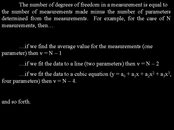
The number of degrees of freedom in a measurement is equal to the number of measurements made minus the number of parameters determined from the measurements. For example, for the case of N measurements, then… …if we find the average value for the measurements (one parameter) then = N – 1 …if we fit the data to a line (two parameters) then = N – 2 …if we fit the data to a cubic equation (y = a 0 + a 1 x + a 2 x 2 + a 3 x 3, four parameters) then = N – 4. and so forth.

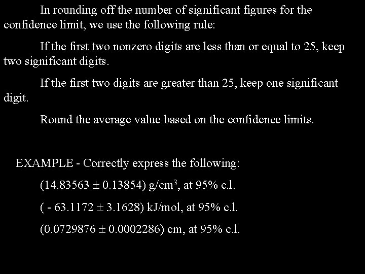
In rounding off the number of significant figures for the confidence limit, we use the following rule: If the first two nonzero digits are less than or equal to 25, keep two significant digits. If the first two digits are greater than 25, keep one significant digit. Round the average value based on the confidence limits. EXAMPLE - Correctly express the following: (14. 83563 0. 13854) g/cm 3, at 95% c. l. ( - 63. 1172 3. 1628) k. J/mol, at 95% c. l. (0. 0729876 0. 0002286) cm, at 95% c. l.

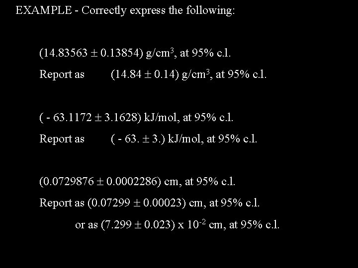
EXAMPLE - Correctly express the following: (14. 83563 0. 13854) g/cm 3, at 95% c. l. Report as (14. 84 0. 14) g/cm 3, at 95% c. l. ( - 63. 1172 3. 1628) k. J/mol, at 95% c. l. Report as ( - 63. 3. ) k. J/mol, at 95% c. l. (0. 0729876 0. 0002286) cm, at 95% c. l. Report as (0. 07299 0. 00023) cm, at 95% c. l. or as (7. 299 0. 023) x 10 -2 cm, at 95% c. l.

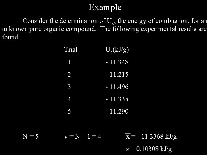
Example Consider the determination of Uc, the energy of combustion, for an unknown pure organic compound. The following experimental results are found N=5 Trial Uc(k. J/g) 1 - 11. 348 2 - 11. 215 3 - 11. 496 4 - 11. 335 5 - 11. 290 =N– 1=4 x = - 11. 3368 k. J/g s = 0. 10308 k. J/g

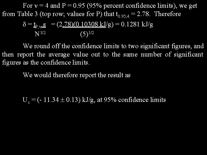
For = 4 and P = 0. 95 (95% percent confidence limits), we get from Table 3 (top row; values for P) that t 0. 95, 4 = 2. 78. Therefore = t. P, s = (2. 78)(0. 10308 k. J/g) = 0. 1281 k. J/g N 1/2 (5)1/2 We round off the confidence limits to two significant figures, and then report the average value out to the same number of significant figures as the confidence limits. We would therefore report the result as Uc = (- 11. 34 0. 13) k. J/g, at 95% confidence limits

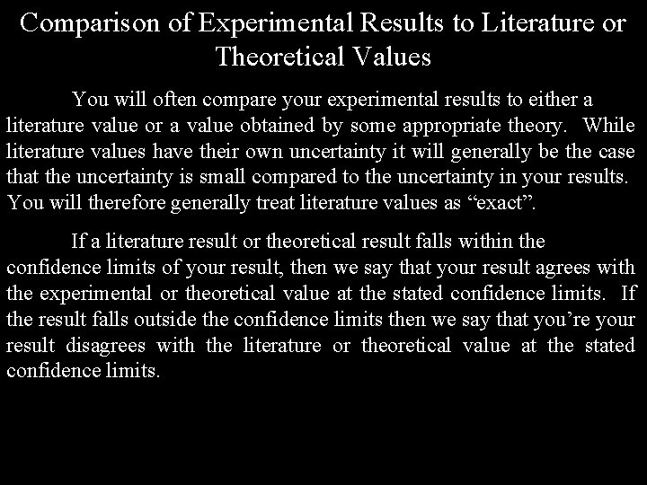
Comparison of Experimental Results to Literature or Theoretical Values You will often compare your experimental results to either a literature value or a value obtained by some appropriate theory. While literature values have their own uncertainty it will generally be the case that the uncertainty is small compared to the uncertainty in your results. You will therefore generally treat literature values as “exact”. If a literature result or theoretical result falls within the confidence limits of your result, then we say that your result agrees with the experimental or theoretical value at the stated confidence limits. If the result falls outside the confidence limits then we say that you’re your result disagrees with the literature or theoretical value at the stated confidence limits.

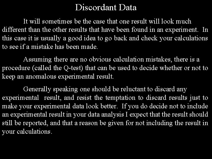
Discordant Data It will sometimes be the case that one result will look much different than the other results that have been found in an experiment. In this case it is usually a good idea to go back and check your calculations to see if a mistake has been made. Assuming there are no obvious calculation mistakes, there is a procedure (called the Q-test) that can be used to decide whether or not to keep an anomalous experimental result. Generally speaking one should be reluctant to discard any experimental result, and resist the temptation to discard results just to make your experimental data look better. If you do decide not to include an experimental result in your data analysis I expect that the result should still be reported, and that a reason be given for not including the result in your calculations.

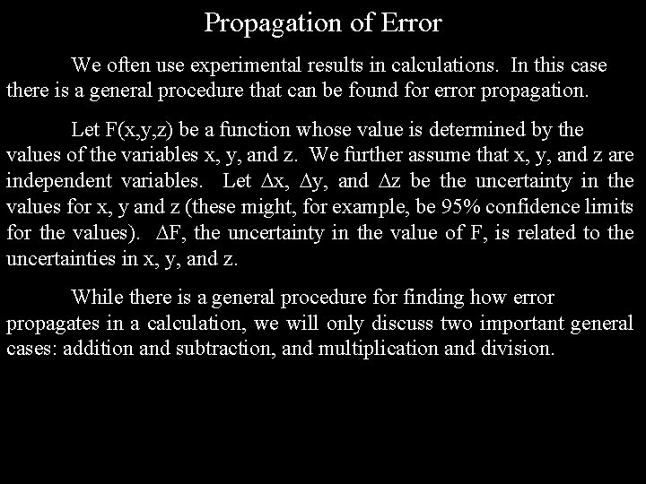
Propagation of Error We often use experimental results in calculations. In this case there is a general procedure that can be found for error propagation. Let F(x, y, z) be a function whose value is determined by the values of the variables x, y, and z. We further assume that x, y, and z are independent variables. Let x, y, and z be the uncertainty in the values for x, y and z (these might, for example, be 95% confidence limits for the values). F, the uncertainty in the value of F, is related to the uncertainties in x, y, and z. While there is a general procedure for finding how error propagates in a calculation, we will only discuss two important general cases: addition and subtraction, and multiplication and division.

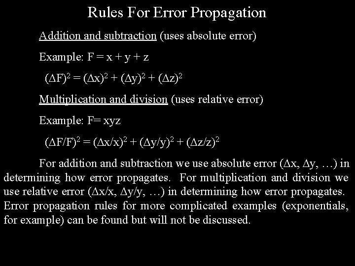
Rules For Error Propagation Addition and subtraction (uses absolute error) Example: F = x + y + z ( F)2 = ( x)2 + ( y)2 + ( z)2 Multiplication and division (uses relative error) Example: F= xyz ( F/F)2 = ( x/x)2 + ( y/y)2 + ( z/z)2 For addition and subtraction we use absolute error ( x, y, …) in determining how error propagates. For multiplication and division we use relative error ( x/x, y/y, …) in determining how error propagates. Error propagation rules for more complicated examples (exponentials, for example) can be found but will not be discussed.

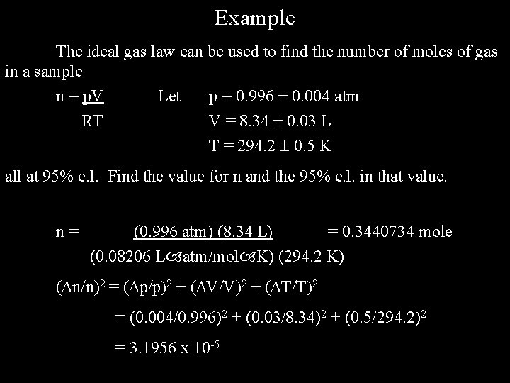
Example The ideal gas law can be used to find the number of moles of gas in a sample n = p. V Let p = 0. 996 0. 004 atm RT V = 8. 34 0. 03 L T = 294. 2 0. 5 K all at 95% c. l. Find the value for n and the 95% c. l. in that value. n= (0. 996 atm) (8. 34 L) = 0. 3440734 mole (0. 08206 L atm/mol K) (294. 2 K) ( n/n)2 = ( p/p)2 + ( V/V)2 + ( T/T)2 = (0. 004/0. 996)2 + (0. 03/8. 34)2 + (0. 5/294. 2)2 = 3. 1956 x 10 -5

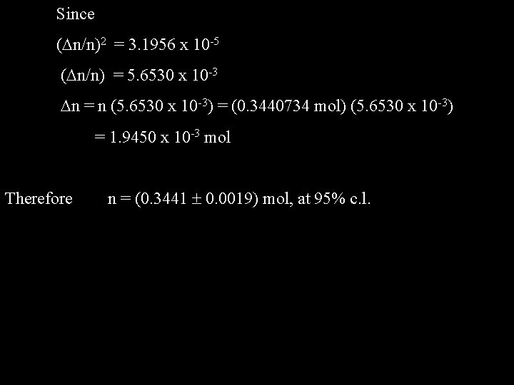
Since ( n/n)2 = 3. 1956 x 10 -5 ( n/n) = 5. 6530 x 10 -3 n = n (5. 6530 x 10 -3) = (0. 3440734 mol) (5. 6530 x 10 -3) = 1. 9450 x 10 -3 mol Therefore n = (0. 3441 0. 0019) mol, at 95% c. l.

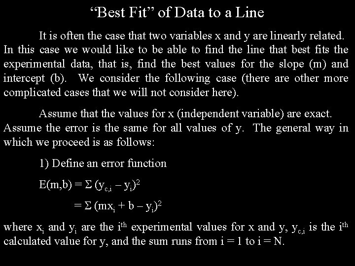
“Best Fit” of Data to a Line It is often the case that two variables x and y are linearly related. In this case we would like to be able to find the line that best fits the experimental data, that is, find the best values for the slope (m) and intercept (b). We consider the following case (there are other more complicated cases that we will not consider here). Assume that the values for x (independent variable) are exact. Assume the error is the same for all values of y. The general way in which we proceed is as follows: 1) Define an error function E(m, b) = (yc, i – yi)2 = (mxi + b – yi)2 where xi and yi are the ith experimental values for x and y, yc, i is the ith calculated value for y, and the sum runs from i = 1 to i = N.

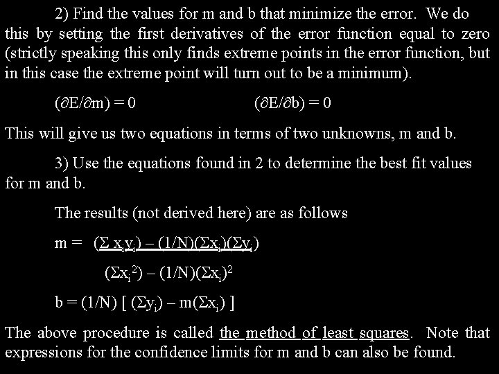
2) Find the values for m and b that minimize the error. We do this by setting the first derivatives of the error function equal to zero (strictly speaking this only finds extreme points in the error function, but in this case the extreme point will turn out to be a minimum). ( E/ m) = 0 ( E/ b) = 0 This will give us two equations in terms of two unknowns, m and b. 3) Use the equations found in 2 to determine the best fit values for m and b. The results (not derived here) are as follows m = ( xiyi) – (1/N)( xi)( yi) ( xi 2) – (1/N)( xi)2 b = (1/N) [ ( yi) – m( xi) ] The above procedure is called the method of least squares. Note that expressions for the confidence limits for m and b can also be found.

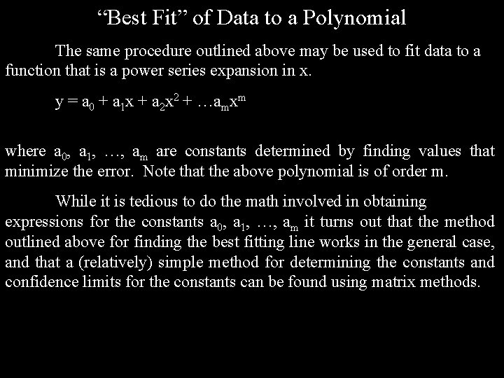
“Best Fit” of Data to a Polynomial The same procedure outlined above may be used to fit data to a function that is a power series expansion in x. y = a 0 + a 1 x + a 2 x 2 + …amxm where a 0, a 1, …, am are constants determined by finding values that minimize the error. Note that the above polynomial is of order m. While it is tedious to do the math involved in obtaining expressions for the constants a 0, a 1, …, am it turns out that the method outlined above for finding the best fitting line works in the general case, and that a (relatively) simple method for determining the constants and confidence limits for the constants can be found using matrix methods.

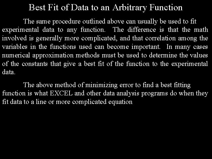
Best Fit of Data to an Arbitrary Function The same procedure outlined above can usually be used to fit experimental data to any function. The difference is that the math involved is generally more complicated, and that correlation among the variables in the functions used can become important. In many cases numerical approximation methods must be used to determine the values of the constants that give a best fit of the function to the experimental data. The above method of minimizing error to find a best fitting function is what EXCEL and other data analysis programs do when they fit data to a line or more complicated equation

References 1) P. R. Bevington, Data Reduction and Error Analysis for the Physical Sciences, Second Edition, (Mc. Graw-Hill, New York, 1992). 2) J. N. Nibler, C. W. Garland, K. J. Stine, J. E. Kim, Experiments in Physical Chemistry, Ninth Edition, (Mc. Graw-Hill, New York, 2014), Chapter 2. 3) R. L. Ott, M. Longnecker, An Introduction to Statistical Methods and Data Analysis, Seventh Edition, (Cengage Learning, Boston, 2015). 4) D. G. Peters, J. M. Hayes, G. M. Hieftje, Chemical Separation and Measurement, (Saunders, Philadelphia, 1974), Chapter 2. 5) D. A. Skoog, D. M. West, F. J. Holler, S. R. Crouch Fundamentals of Analytical Chemistry, Ninth Edition, (Saunders, Philadelphia, 2013).