Autocorrelation image processing for shear analysis in weak

Autocorrelation image processing for shear analysis in weak lensing Paul Stankus, ORNL BNL Astro Group Meeting, 3 November 2015

Physics and shear Cause: (e 1, e 2) derivatives of gravitational lensing potential Effect: = b a θ

Life in (e 1, e 2) space e = 0. 25, 0. 8 Measure (e 1, e 2) of galaxy images Estimators of induced gravitational shear

Wish list? Can we find an image processing technique that will let us • Push every image toward a known fit-able shape, while still preserving eccentricity information • Take advantage of the properties of pixel by pixel noise (whiter shade of pale)

Convolutions/Correlations Two interesting, suggestive mathematical facts: • Repeated auto-correlation/convolution converges toward a Gaussian, while preserving variance ratios • Auto-correlation of white noise is a predictable δ() function

Image processing, first order Original Auto convolution Auto correlation

Image processing, first order Original Auto convolution Auto correlation

Successive autocorrelation Original First auto correlation Second auto correlation

Main Message: These are hard to fit, requiring a large “model space” These are easy to fit, requiring a small “model space”

Example: Poor Man’s Barred Spiral A galaxy-like image made from the sum of two Gaussians Non-elliptical objects have no single, unambiguous intrinsic ellipticity But all we require is a shear estimator

Shear Estimators Take any image, and rotate it in many steps from 0 -π Shear each rotated image by the same given amount A good shear estimator for each image, returns the induced shear when averaged over all rotations

Shear recovery Each rotated image was sheared by {e 1, e 2}={0. 1, 0}, and the circle-averaged shear estimator recovers that

The challenge: noise and PSF Two true facts: (1) Any auto-correlate of an image has the same shear transformation properties as images do (2) If an observed image is the convolution of an original and a PSF, then its autocorrelate is the convolution of the original image autocorrelate and the PSF autocorrelate

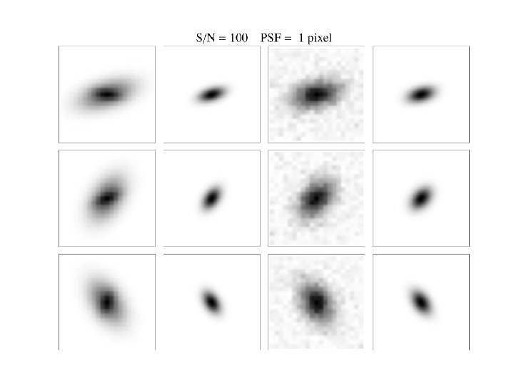
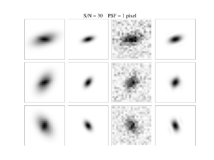
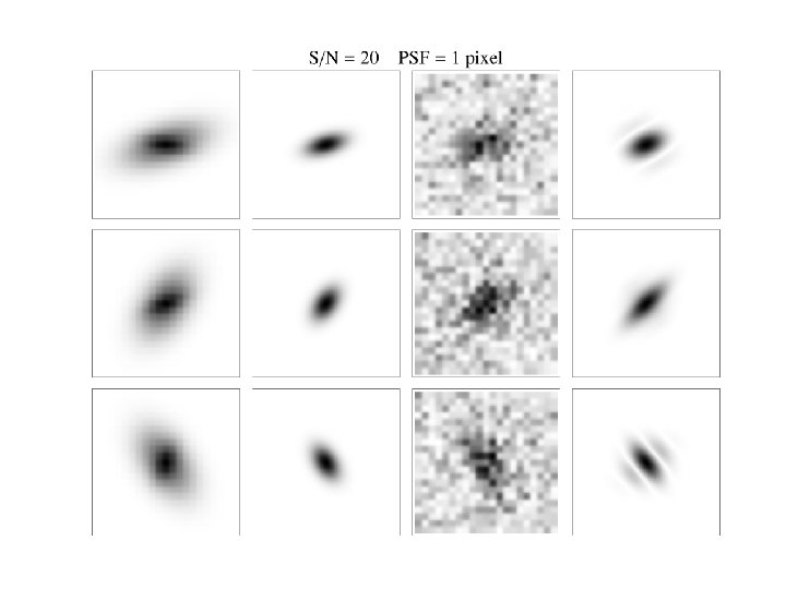
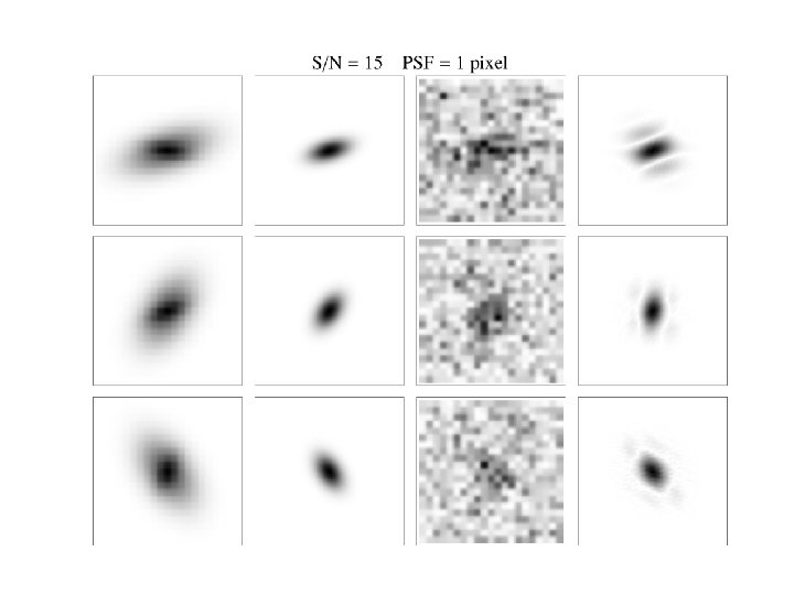
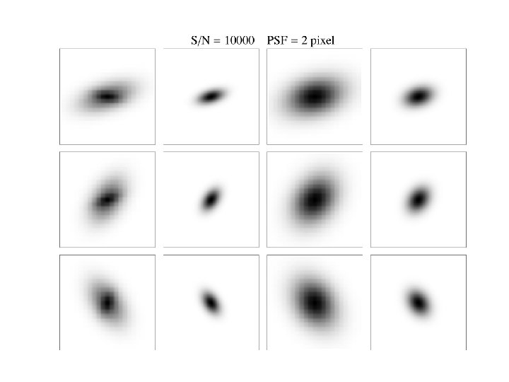
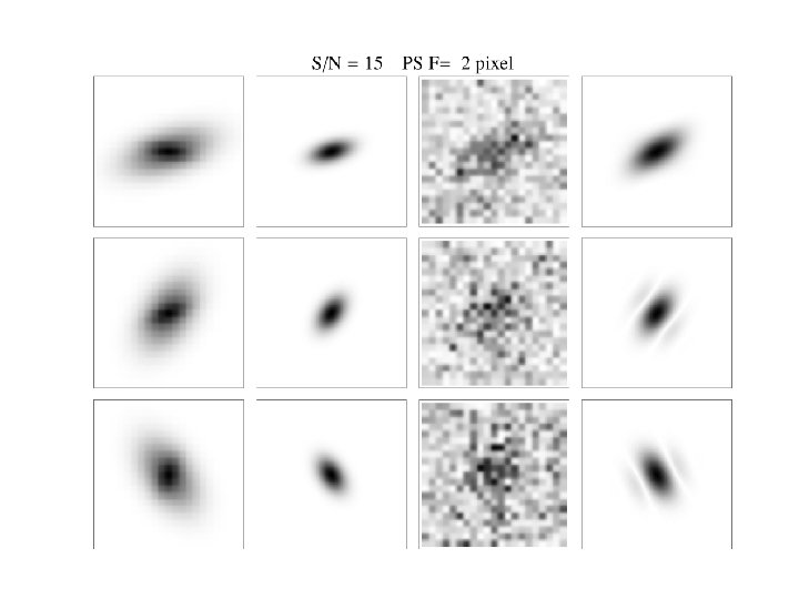
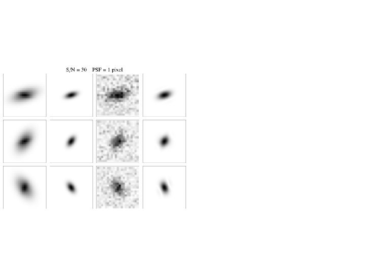
Original, rotated & sheared Second autocorrelate Add PSF and noise Second autocorrelate

“Quickie” PSF correction Fit central “cap” of second autocorrelate with elliptical form, extract (e, θ, scale) Convert (e, θ, scale) to Gaussian-equivalent “faux-variance” matrix No PSF Translate faux-variance back into equivalent ellipticity (e, θ, scale) Report e as shear estimator Subtract moments of PSF autocorrelate from fauxvariance

Black: No PSF applied Red: PSF applied and corrected Green: PSF applied but not corrected

Black: No PSF applied Red: PSF applied and corrected Green: PSF applied but not corrected

S/N = 100 PSF 1. 0 Pixel 1. 4 Pixel 2. 0 Pixel 30 20 15

Summary • In principle the autocorrelate has the same shear transform and PSF properties as an image • In practice the autocorrelate results in a smooth profile, readily fit-able and preserving ellipticity even in the worst noise conditions • Excellent noise resistance for shear estimator in absence of PSF • With “quickie” faux-variance scheme, see very good PSF correction performance right out of the box before any optimizations or corrections

Central “cap” preserves ellipticity Original Fit Here Second auto correlation

Fitting > Moments How do we go from an image to measures of (e 1, e 2) estimators? Two basic approaches: Moments: e. g. covariance matrix • No assumption of detailed galaxy shape • Bias from clipping in tails • Bad noise performance, or use weighting (unknown, tricky) Fitting: with parameterized form • Works on any piece of image • Better noise resistance; but potential noise bias • True shapes unknown; noise effect depends on shape (Great 3)

Four experiments: Using auto-correlation/convolution + fitting technique: • Look at three very different images with same eccentricity, see how noise performance varies • Look at noise behavior at high ellipticity • Using Gaussian images, look at resistance to tail clipping • Shear an assortment of Gaussians, look at shear recovery on average

E 1: Meet our contestants DISH NGC 4414 RMN 1970

E 1: Meet our contestants DISH NGC 4414 RMN 1970

Image processing, second order Original First auto correlation Second auto correlation

Image processing, first order Original Auto convolution Auto correlation