Neighborhood Processing Basic Image Processing Operations Neighborhood processing

Neighborhood Processing

Basic Image Processing Operations • Neighborhood processing • process the pixel with its neighbors • Point operations • process according to the pixel’s value alone.

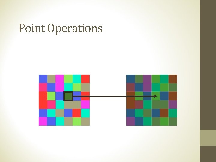
Point Operations

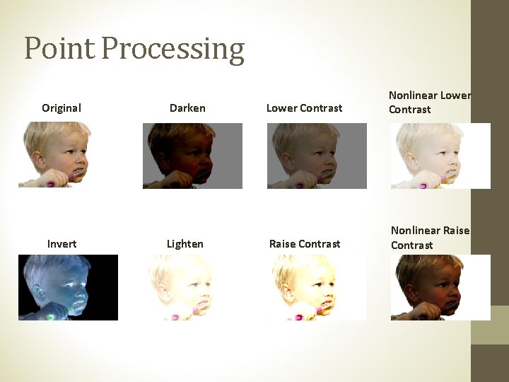
Point Processing Original Invert Darken Lighten Lower Contrast Nonlinear Lower Contrast Raise Contrast Nonlinear Raise Contrast

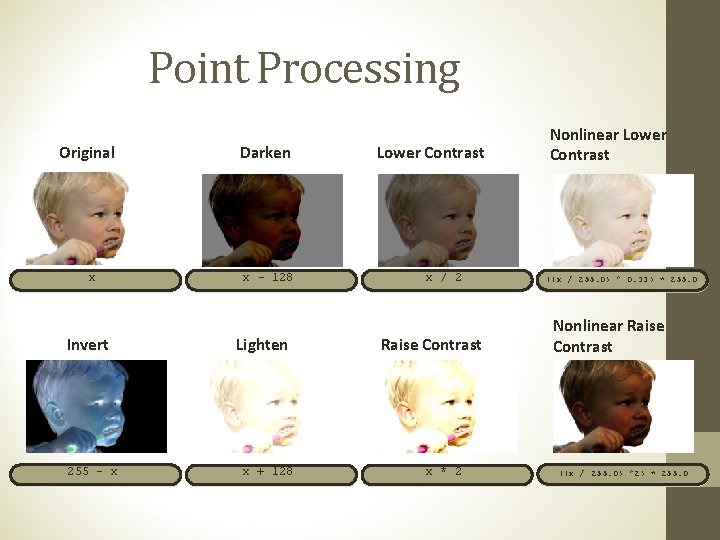
Point Processing Original x Invert 255 - x Darken x - 128 Lighten x + 128 Lower Contrast x / 2 Raise Contrast x * 2 Nonlinear Lower Contrast ((x / 255. 0) ^ 0. 33) * 255. 0 Nonlinear Raise Contrast ((x / 255. 0) ^2) * 255. 0

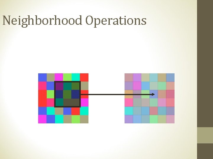
Neighborhood Operations

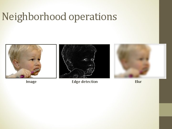
Neighborhood operations Image Edge detection Blur

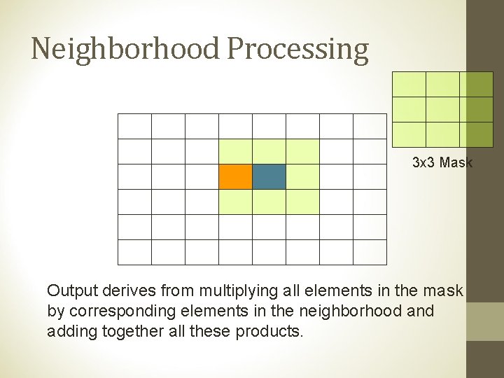
Neighborhood Processing 3 x 3 Mask Output derives from multiplying all elements in the mask by corresponding elements in the neighborhood and adding together all these products.

Filter • A rule or procedure for processing an image • Combination of mask and function • Goal: separating/attenuating a desired component of an observed image • Type: • Linear (function), Nonlinear (function) • Low-pass filter (LPF), High-pass filter (HPF), Band-pass filter (BPF)

Steps of Linear Spatial Filtering • Position the mask over the current pixel. • Form all products of filter elements with the corresponding elements of the neighborhood. • Add all products. • Other names for mask: filter, mask, filter mask, kernel, template or etc. window,

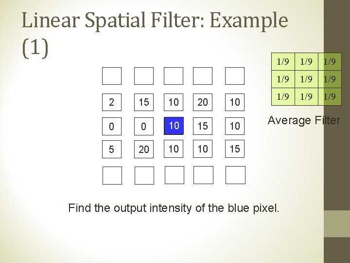
Linear Spatial Filter: Example (1) 1/9 1/9 1/9 2 15 10 20 10 0 0 10 15 10 5 20 10 10 15 Average Filter Find the output intensity of the blue pixel.

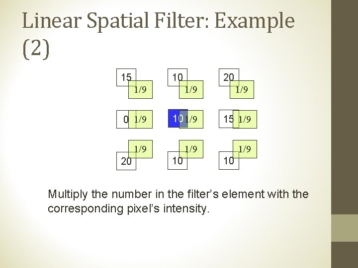
Linear Spatial Filter: Example (2) 15 10 20 1/9 1/9 0 1/9 15 1/9 1/9 20 10 10 Multiply the number in the filter’s element with the corresponding pixel’s intensity.

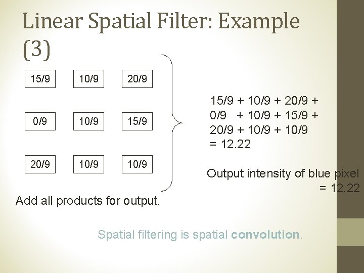
Linear Spatial Filter: Example (3) 15/9 10/9 20/9 10/9 15/9 20/9 10/9 Add all products for output. 15/9 + 10/9 + 20/9 + 10/9 + 15/9 + 20/9 + 10/9 = 12. 22 Output intensity of blue pixel = 12. 22 Spatial filtering is spatial convolution.

Break Sholat sampai 12: 47

Correlation and Convolution of Digital Image

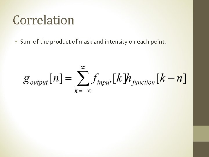
Correlation • Sum of the product of mask and intensity on each point.

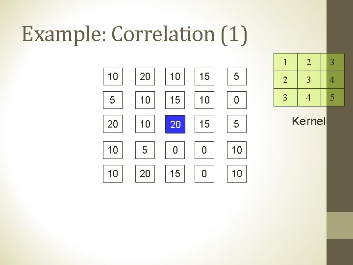
Example: Correlation (1) 1 2 3 10 20 10 15 5 2 3 4 5 10 15 10 0 3 4 5 20 10 20 15 5 10 5 0 0 10 10 20 15 0 10 Kernel

Example: Correlation (2) 10 15 10 1 2 3 10 2 20 3 15 4 3 4 5 5 0 0 Multiply and sum all products. 10 1 +15 2 +10 3 +10 2 +20 3 +15 4 +5 3 +0 4 +0 5 = 225

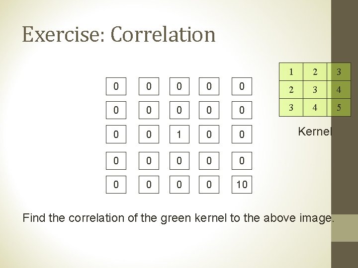
Exercise: Correlation 1 2 3 0 0 0 2 3 4 0 0 0 3 4 5 0 0 1 0 0 0 10 Kernel Find the correlation of the green kernel to the above image.

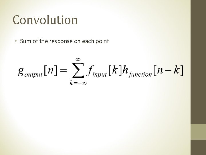
Convolution • Sum of the response on each point

Example: Convolution (1) 5 4 3 10 20 10 15 5 4 3 2 5 10 15 10 0 3 2 1 20 10 20 15 5 10 5 0 0 10 10 20 15 0 10 Reverse Kernel!! 1 2 3 4 3 4 5 Kernel

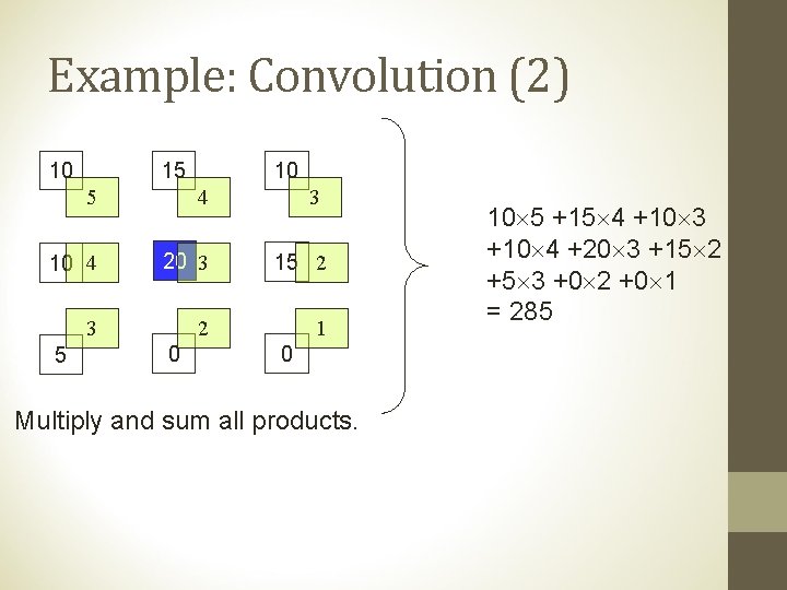
Example: Convolution (2) 10 15 10 5 4 3 10 4 20 3 15 2 3 2 1 5 0 0 Multiply and sum all products. 10 5 +15 4 +10 3 +10 4 +20 3 +15 2 +5 3 +0 2 +0 1 = 285

Exercise: Convolution 1 2 3 0 0 0 2 3 4 0 0 0 3 4 5 0 0 1 0 0 0 10 Kernel Find the convolution of the green kernel to the above image.

Filtering the Image

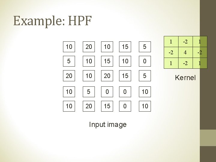
Example: HPF 10 20 10 15 5 5 10 15 10 0 20 15 5 10 5 0 0 10 10 20 15 0 10 Input image 1 -2 4 -2 1 Kernel

Example: HPF (2) 10 20 10 15 5 5 0 20 -10 0 20 -40 25 15 5 10 5 -35 0 10 10 20 15 0 10 Filtered Image

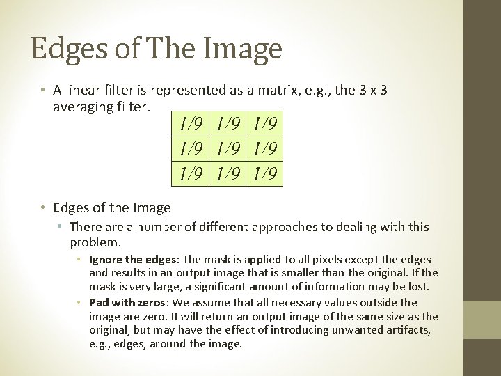
Edges of The Image • A linear filter is represented as a matrix, e. g. , the 3 x 3 averaging filter. 1/9 1/9 1/9 • Edges of the Image • There a number of different approaches to dealing with this problem. • Ignore the edges: The mask is applied to all pixels except the edges and results in an output image that is smaller than the original. If the mask is very large, a significant amount of information may be lost. • Pad with zeros: We assume that all necessary values outside the image are zero. It will return an output image of the same size as the original, but may have the effect of introducing unwanted artifacts, e. g. , edges, around the image.

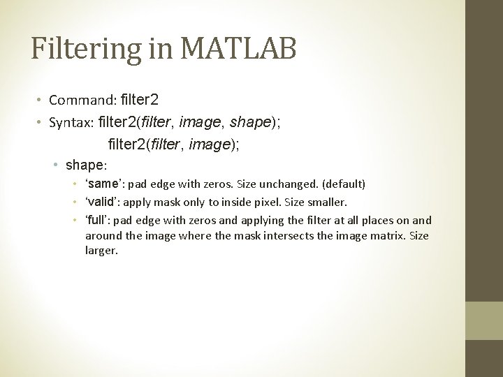
Filtering in MATLAB • Command: filter 2 • Syntax: filter 2(filter, image, shape); filter 2(filter, image); • shape: • ‘same’: pad edge with zeros. Size unchanged. (default) • ‘valid’: apply mask only to inside pixel. Size smaller. • ‘full’: pad edge with zeros and applying the filter at all places on and around the image where the mask intersects the image matrix. Size larger.

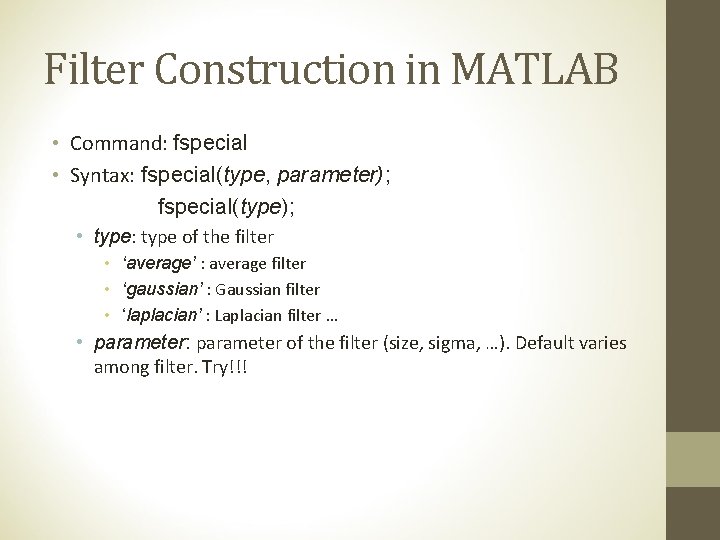
Filter Construction in MATLAB • Command: fspecial • Syntax: fspecial(type, parameter); fspecial(type); • type: type of the filter • ‘average’ : average filter • ‘gaussian’ : Gaussian filter • ‘laplacian’ : Laplacian filter … • parameter: parameter of the filter (size, sigma, …). Default varies among filter. Try!!!

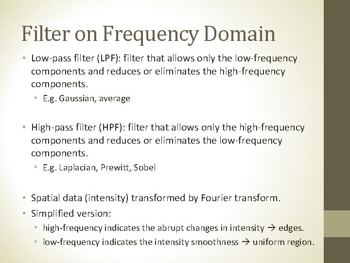
Filter on Frequency Domain • Low-pass filter (LPF): filter that allows only the low-frequency components and reduces or eliminates the high-frequency components. • E. g. Gaussian, average • High-pass filter (HPF): filter that allows only the high-frequency components and reduces or eliminates the low-frequency components. • E. g. Laplacian, Prewitt, Sobel • Spatial data (intensity) transformed by Fourier transform. • Simplified version: • high-frequency indicates the abrupt changes in intensity edges. • low-frequency indicates the intensity smoothness uniform region.

Computing Consideration • Filter may lead to the value outside [0, 255] • Solution 1: Make negative values positive (use absolute value) good when there are few negative values and the negative values are close to zero • Solution 2: Clip values. Values larger than 255 become 255 and values less than 0 become 0. not good if there are many values outside the range. • Solution 3: Scaling transformation. Rescale the range to [0, 255] by pixel transform. Suppose g. L and g. H are the lowest and the highest values.

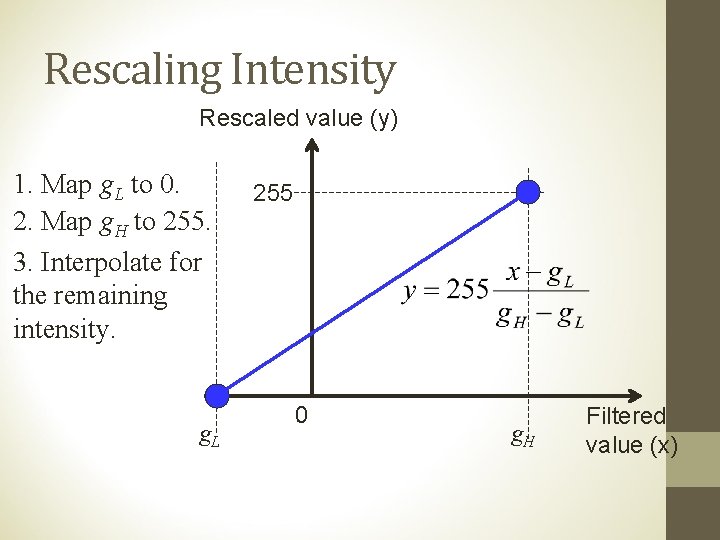
Rescaling Intensity Rescaled value (y) 1. Map g. L to 0. 2. Map g. H to 255. 3. Interpolate for the remaining intensity. g. L 255 0 g. H Filtered value (x)

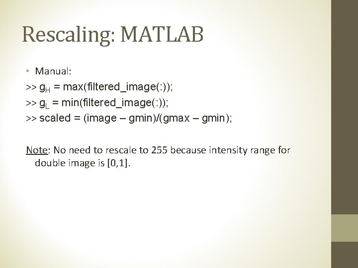
Rescaling: MATLAB • Manual: >> g. H = max(filtered_image(: )); >> g. L = min(filtered_image(: )); >> scaled = (image – gmin)/(gmax – gmin); Note: No need to rescale to 255 because intensity range for double image is [0, 1].

Rescaling: MATLAB (2) • Command: mat 2 gray • Syntax: mat 2 gray(double_image); What this command do? • scale the value in double_image to displayable value. Output is double type. • minimum value is mapped to 0. • maximum value is mapped to 1.

Low Pass Filter Averaging Smoothing

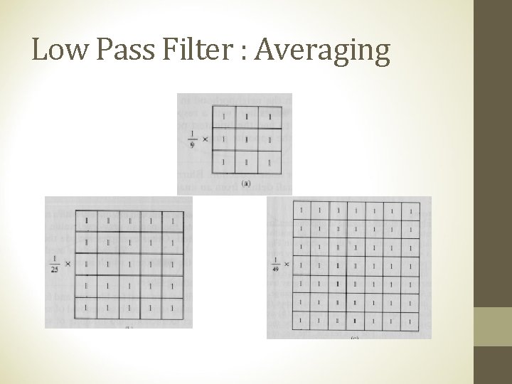
Low Pass Filter • Useful for reducing noise and eliminating small details. • The elements of the mask must be positive. • Sum of mask elements is 1 (after normalization). Gaussian

Low Pass Filter : Averaging

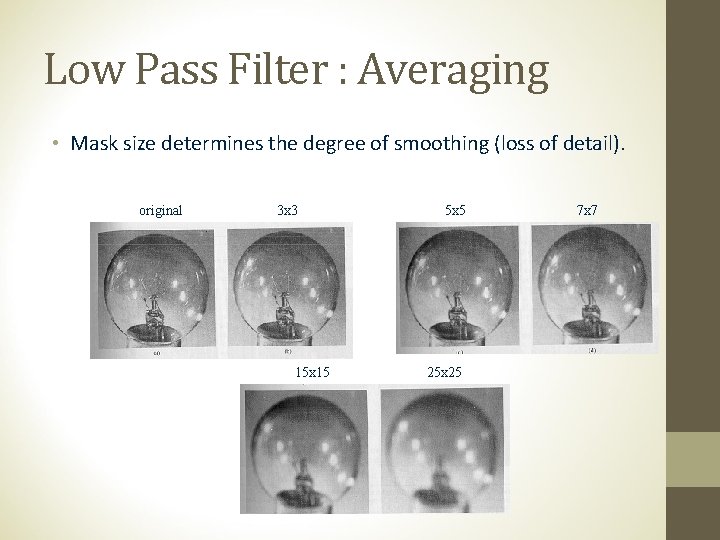
Low Pass Filter : Averaging • Mask size determines the degree of smoothing (loss of detail). original 3 x 3 15 x 15 5 x 5 25 x 25 7 x 7

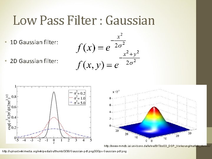
Low Pass Filter : Gaussian • 1 D Gaussian filter: • 2 D Gaussian filter: http: //www-mmdb. iai. uni-bonn. de/lehre/BIT/ss 03_DSP_Vorlesung/matlab_demos/ http: //upload. wikimedia. org/wikipedia/su/thumb/3/38/Gaussian-pdf. png/300 px-Gaussian-pdf. png

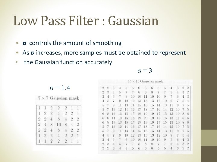
Low Pass Filter : Gaussian • σ controls the amount of smoothing • As σ increases, more samples must be obtained to represent • the Gaussian function accurately. σ=3 σ = 1. 4

Benefits of Gaussian Filter • They are mathematically very well behaved. The Fourier transform of a Gaussian filter is another Gaussian. • There are rotationally symmetric, so are very good starting points for some edge-detection algorithms. • They are separable in x and y axes. This can lead to very fast implementations. • The convolution of two Gaussians is another Gaussian.

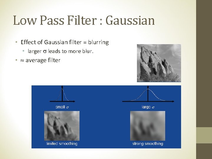
Low Pass Filter : Gaussian • Effect of Gaussian filter = blurring • larger leads to more blur. • average filter

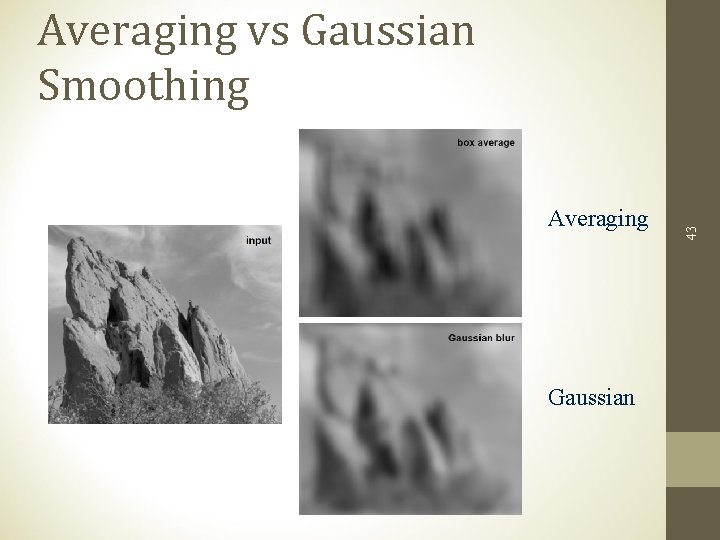
Averaging Gaussian 43 Averaging vs Gaussian Smoothing

Gaussian Filter: MATLAB • Construction of Gaussian filter: • command: fspecial(‘gaussian’, size, gamma); size : size of the filter [row column], default [3 3] gamma : , default 0. 5. >>gaussian 1 = fspecial(‘gaussian’, [5 5], 5); Create the 5 5 Gaussian filter with the value of 5. >>gaussian 2 = fspecial(‘gaussian’, 3, 0. 75); Create the 3 3 Gaussian filter with the value of 0. 75. TRY !!

High Pass Filter Edge Sharpening

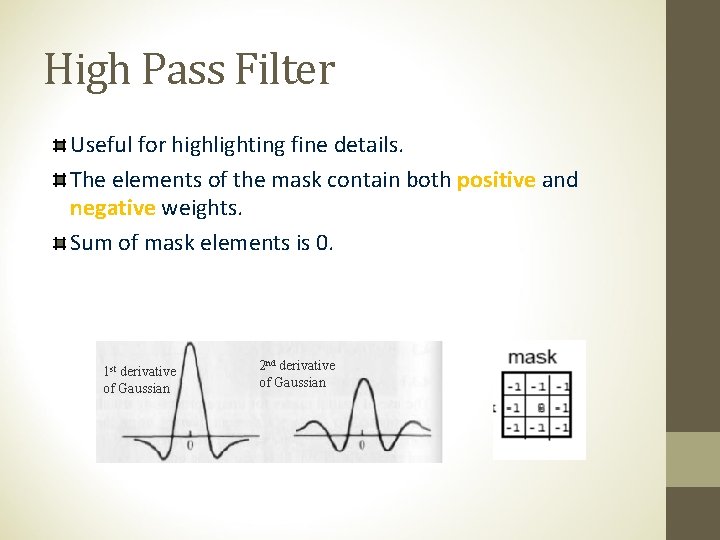
High Pass Filter Useful for highlighting fine details. The elements of the mask contain both positive and negative weights. Sum of mask elements is 0. 1 st derivative of Gaussian 2 nd derivative of Gaussian

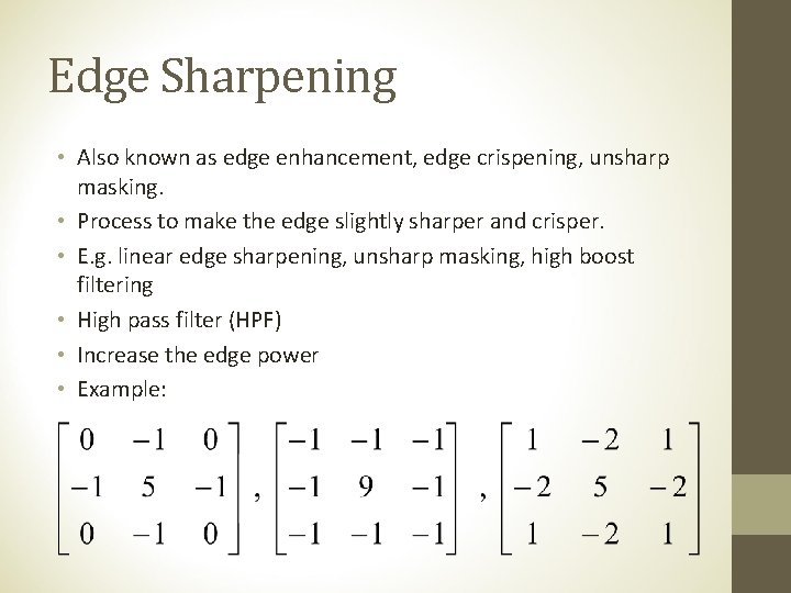
Edge Sharpening • Also known as edge enhancement, edge crispening, unsharp masking. • Process to make the edge slightly sharper and crisper. • E. g. linear edge sharpening, unsharp masking, high boost filtering • High pass filter (HPF) • Increase the edge power • Example:

High Pass Filter : MATLAB • Command: filter 2 • Syntax: filter 2(filter, image, shape); filter 2(filter, image); • shape: • ‘same’: pad edge with zeros. Size unchanged. (default) • ‘valid’: apply mask only to inside pixel. Size smaller. • ‘full’: pad edge with zeros and applying the filter at all places on and around the image where the mask intersects the image matrix. Size larger. TRY !!

Unsharp Masking and High Boost Filter

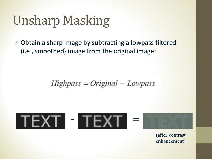
Unsharp Masking • Obtain a sharp image by subtracting a lowpass filtered (i. e. , smoothed) image from the original image: - = (after contrast enhancement)

Unsharp Filter [unsharp_image] = [input] – (a [filter] [input]) = (I* – a [filter]) [input] = [unsharp_filter] [input] I* : matrix whose center member is 1 and the others are zero. E. g. for 3 3 matrix I* = • For 3 3 matrix, after some rearranging term: [unsharp_filter] = MATLAB use this format with the default of 0. 2.

Unsharp Filter: MATLAB • Command: fspecial • Syntax: fspecial(‘unsharp’, alpha); • alpha : alpha value for unsharp filter • Size of the filter is fixed to 3 3 TRY !!

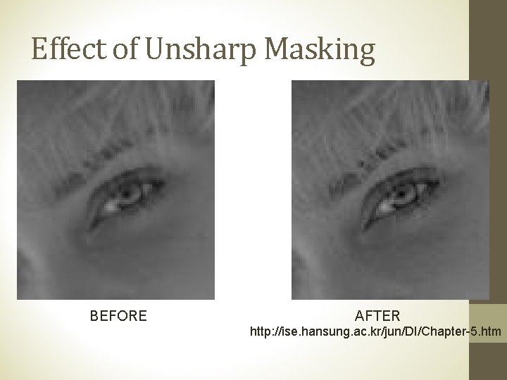
Effect of Unsharp Masking BEFORE AFTER http: //ise. hansung. ac. kr/jun/DI/Chapter-5. htm

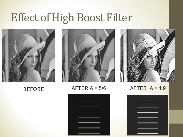
Effect of High Boost Filter BEFORE AFTER A = 5/6 AFTER A = 1. 9

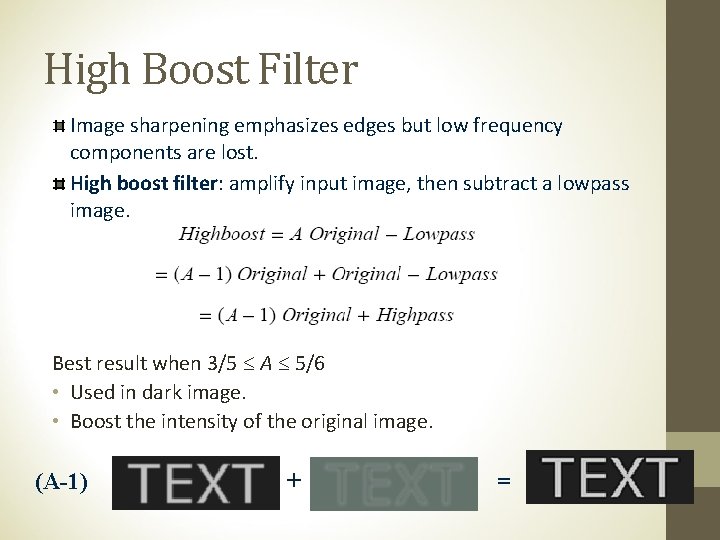
High Boost Filter Image sharpening emphasizes edges but low frequency components are lost. High boost filter: amplify input image, then subtract a lowpass image. Best result when 3/5 A 5/6 • Used in dark image. • Boost the intensity of the original image. (A-1) + =

High Boost Filter : MATLAB TRY AT HOME !!

Image Gradient Edge Detection

Image Derivatives • How can we differentiate a digital image F[x, y]? – Option 1: reconstruct a continuous image, f, then compute the derivative – Option 2: take discrete derivative (finite difference) How would you implement this as a linear filter? : 1 -1 : -1 1

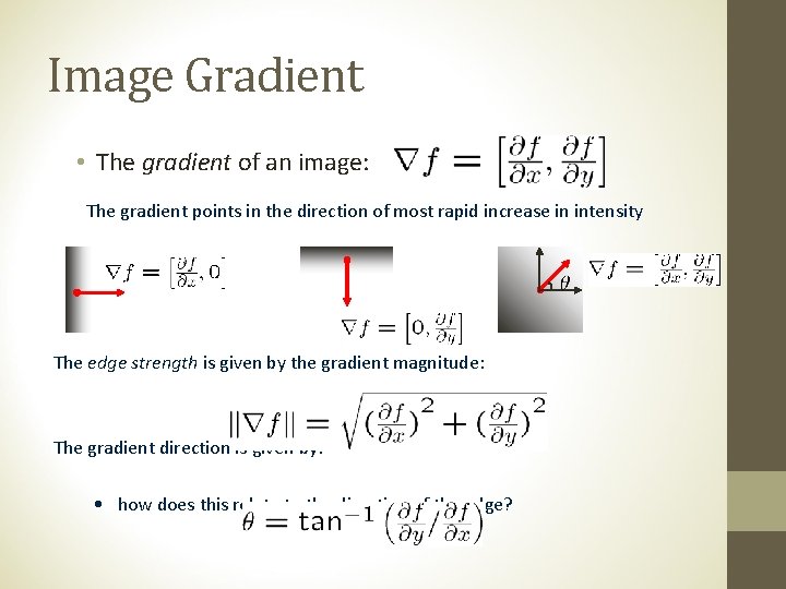
Image Gradient • The gradient of an image: The gradient points in the direction of most rapid increase in intensity The edge strength is given by the gradient magnitude: The gradient direction is given by: • how does this relate to the direction of the edge?

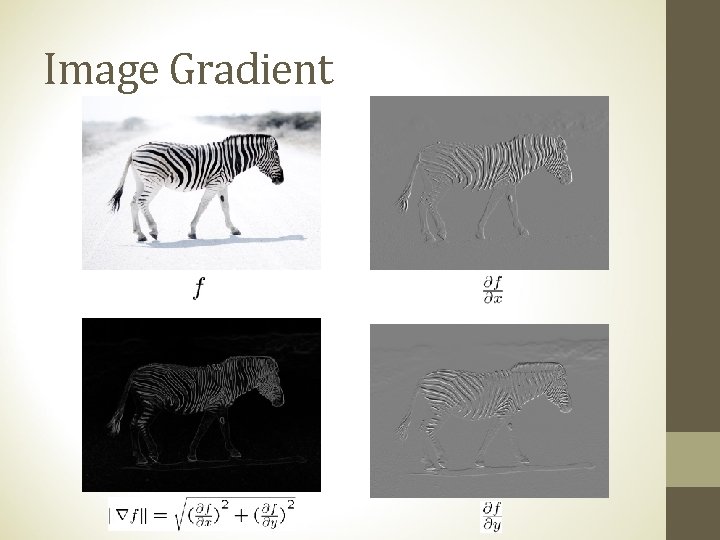
Image Gradient

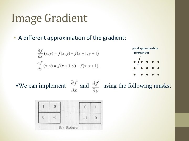
Image Gradient • A different approximation of the gradient: good approximation (x+1/2, y+1/2) * • We can implement and using the following masks:

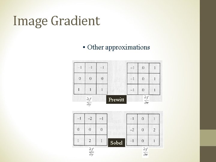
Image Gradient • Other approximations Prewitt Sobel

Image Gradient : MATLAB • Command: fspecial • Syntax: • fspecial(‘prewitt’); • fspecial (‘sobel’); TRY !!

Tugas Individu Coba Praktekkan Filter • High Pass Filter • Low Pass Filter • Unsharp Masking • High Boos Filter • Image Gradient pada citra digital bebas dengan MATLAB. Tampilkan kode, hasil citra dan analisisnya pada file docx, kirimkan ke email anbarsanti@yahoo. com paling lambat Selasa, 27 September pukul 07: 00. Selamat Mencoba