Wavelets Transform Multiresolution Analysis Why transform Image representation

Wavelets Transform & Multiresolution Analysis

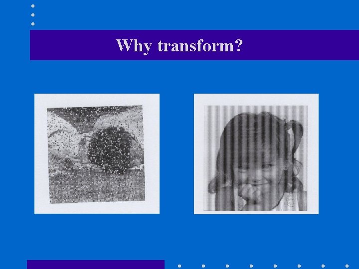
Why transform?

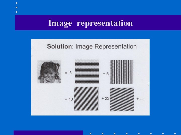
Image representation

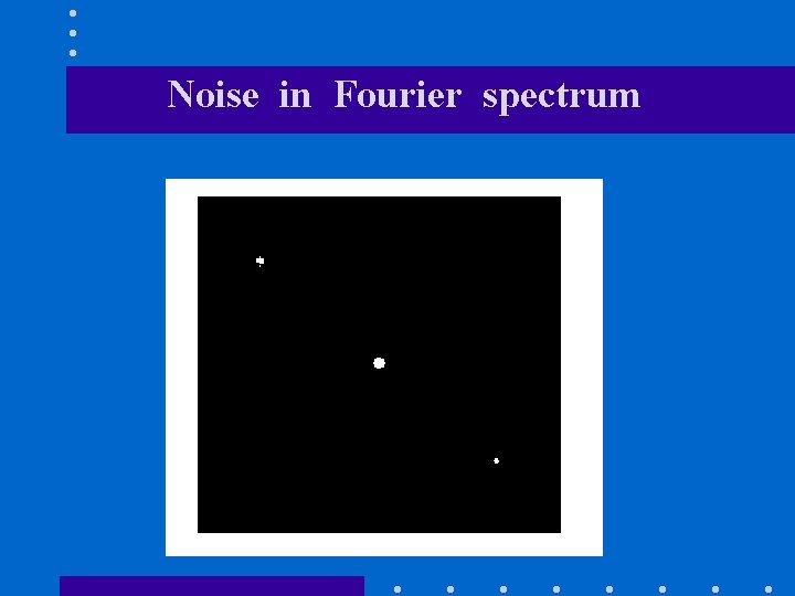
Noise in Fourier spectrum

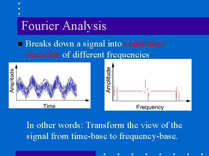
Fourier Analysis n Breaks down a signal into constituent sinusoids of different frequencies In other words: Transform the view of the signal from time-base to frequency-base.

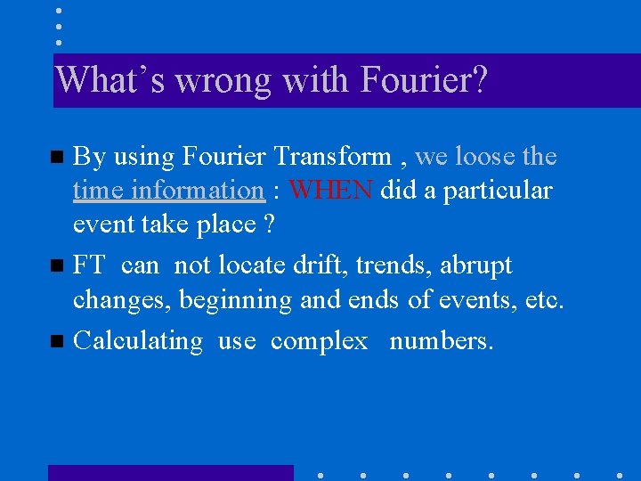
What’s wrong with Fourier? By using Fourier Transform , we loose the time information : WHEN did a particular event take place ? n FT can not locate drift, trends, abrupt changes, beginning and ends of events, etc. n Calculating use complex numbers. n

Time and Space definition • Time – for one dimension waves we start point shifting from source to end in time scale. • Space – for image point shifting is two dimensional. • Here they are synonyms.

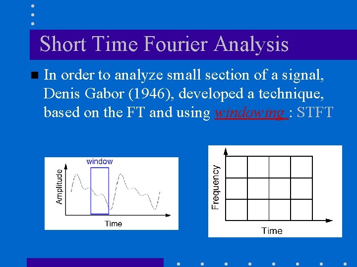
Short Time Fourier Analysis n In order to analyze small section of a signal, Denis Gabor (1946), developed a technique, based on the FT and using windowing : STFT

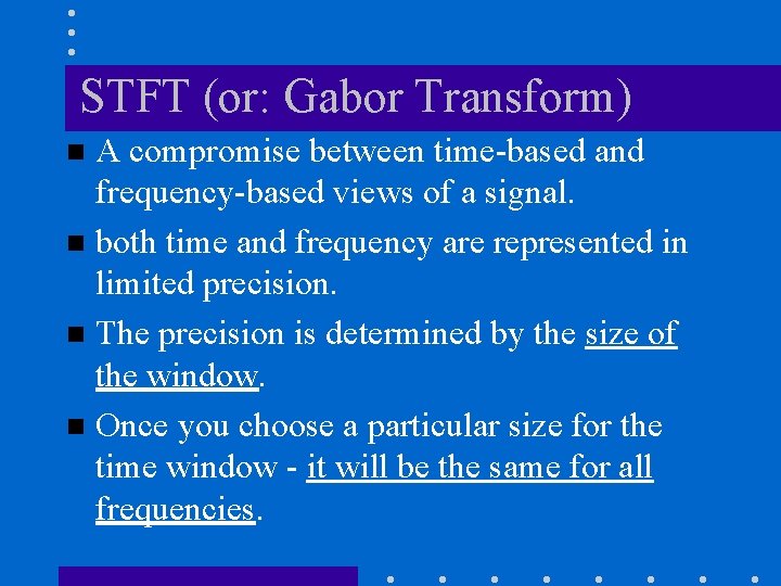
STFT (or: Gabor Transform) A compromise between time-based and frequency-based views of a signal. n both time and frequency are represented in limited precision. n The precision is determined by the size of the window. n Once you choose a particular size for the time window - it will be the same for all frequencies. n

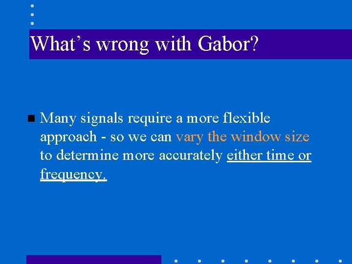
What’s wrong with Gabor? n Many signals require a more flexible approach - so we can vary the window size to determine more accurately either time or frequency.

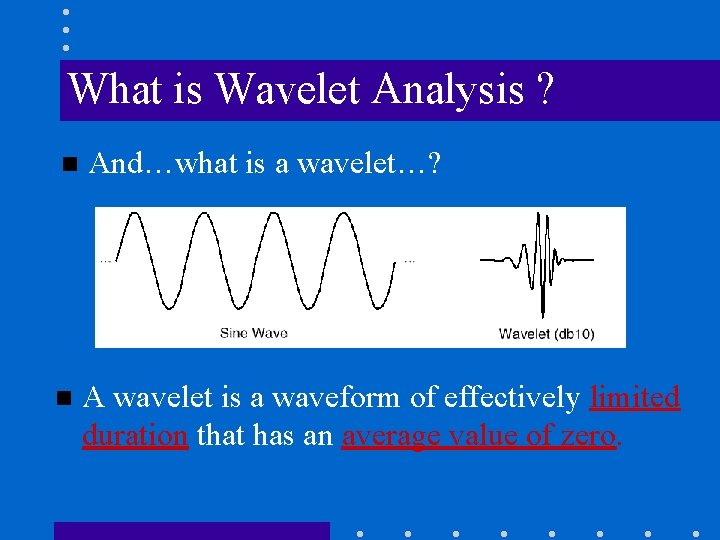
What is Wavelet Analysis ? n And…what is a wavelet…? n A wavelet is a waveform of effectively limited duration that has an average value of zero.

Wavelet's properties • Short time localized waves with zero integral value. • Possibility of time shifting. • Flexibility.

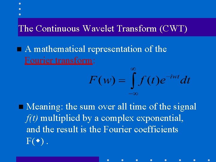
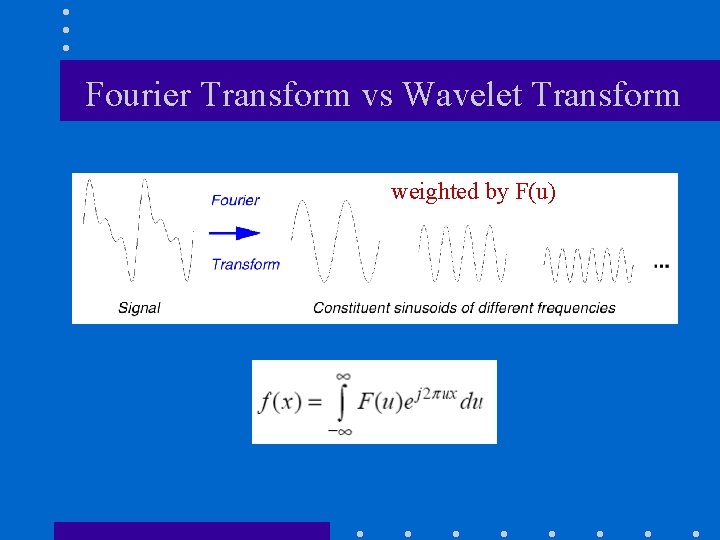
The Continuous Wavelet Transform (CWT) n A mathematical representation of the Fourier transform: n Meaning: the sum over all time of the signal f(t) multiplied by a complex exponential, and the result is the Fourier coefficients F( ).

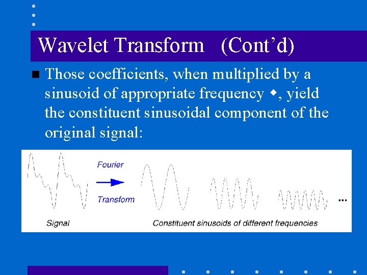
Wavelet Transform (Cont’d) n Those coefficients, when multiplied by a sinusoid of appropriate frequency , yield the constituent sinusoidal component of the original signal:

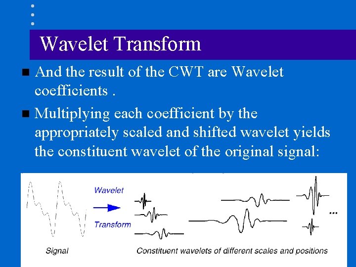
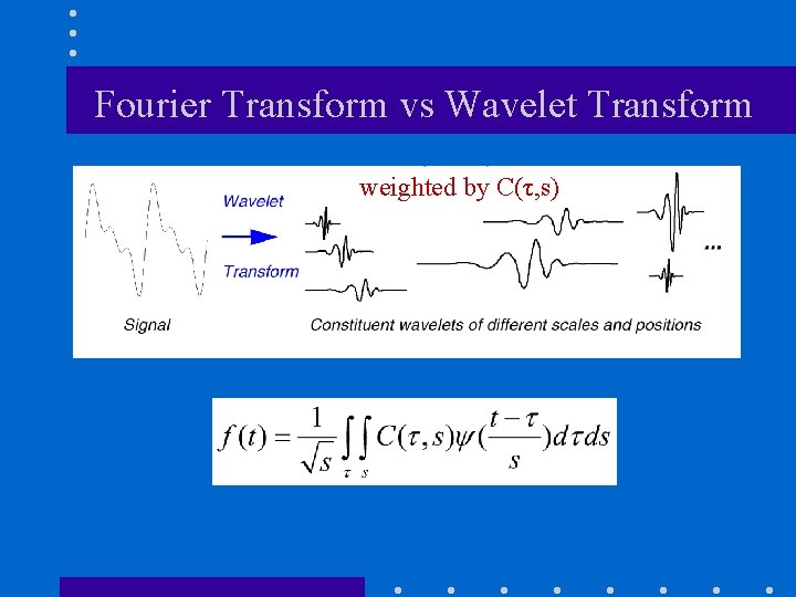
Wavelet Transform And the result of the CWT are Wavelet coefficients. n Multiplying each coefficient by the appropriately scaled and shifted wavelet yields the constituent wavelet of the original signal: n

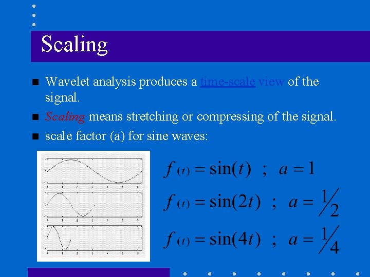
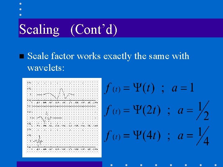
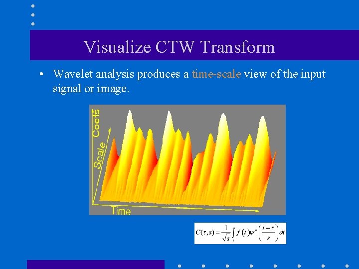
Scaling n n n Wavelet analysis produces a time-scale view of the signal. Scaling means stretching or compressing of the signal. scale factor (a) for sine waves:

Scaling (Cont’d) n Scale factor works exactly the same with wavelets:

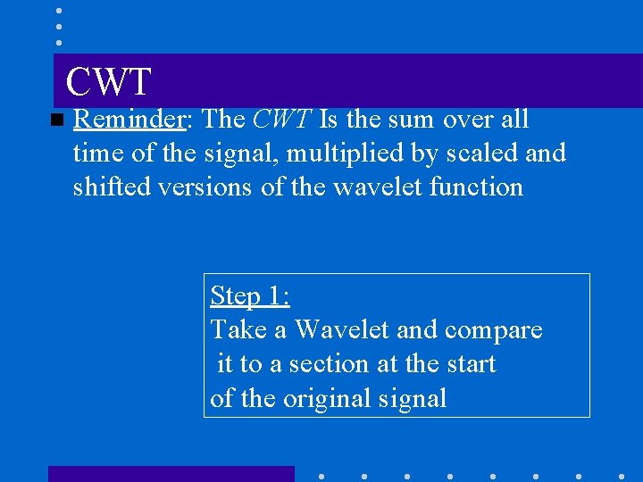
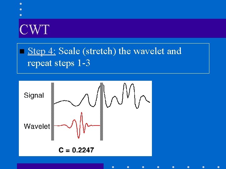
CWT n Reminder: The CWT Is the sum over all time of the signal, multiplied by scaled and shifted versions of the wavelet function Step 1: Take a Wavelet and compare it to a section at the start of the original signal

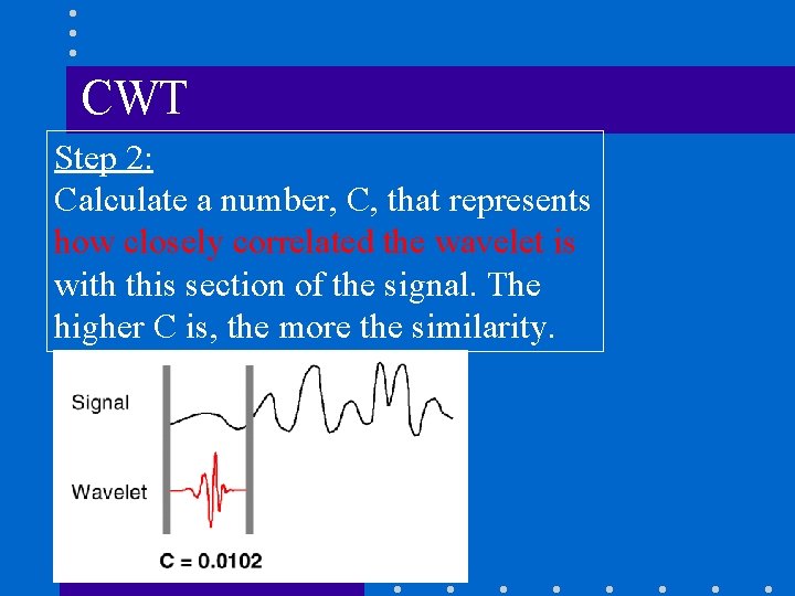
CWT Step 2: Calculate a number, C, that represents how closely correlated the wavelet is with this section of the signal. The higher C is, the more the similarity.

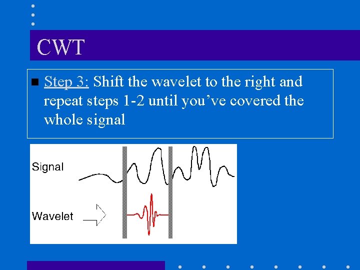
CWT n Step 3: Shift the wavelet to the right and repeat steps 1 -2 until you’ve covered the whole signal

CWT n Step 4: Scale (stretch) the wavelet and repeat steps 1 -3

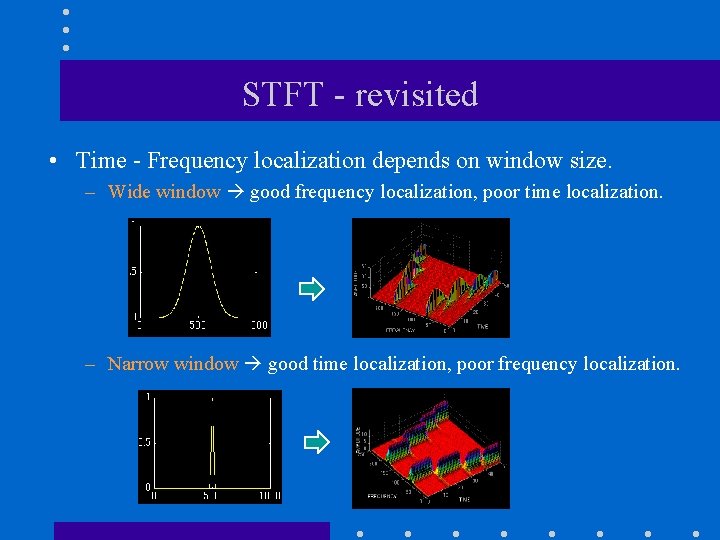
STFT - revisited • Time - Frequency localization depends on window size. – Wide window good frequency localization, poor time localization. – Narrow window good time localization, poor frequency localization.

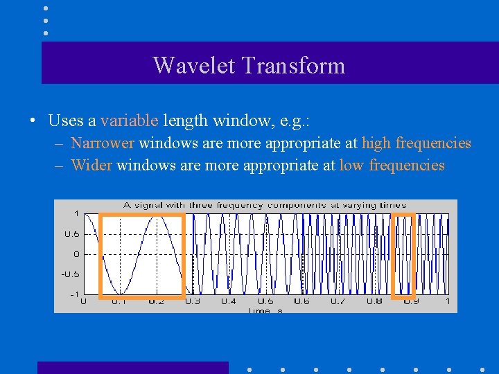
Wavelet Transform • Uses a variable length window, e. g. : – Narrower windows are more appropriate at high frequencies – Wider windows are more appropriate at low frequencies

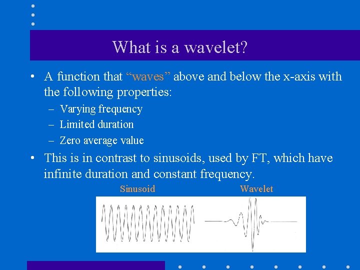
What is a wavelet? • A function that “waves” above and below the x-axis with the following properties: – Varying frequency – Limited duration – Zero average value • This is in contrast to sinusoids, used by FT, which have infinite duration and constant frequency. Sinusoid Wavelet

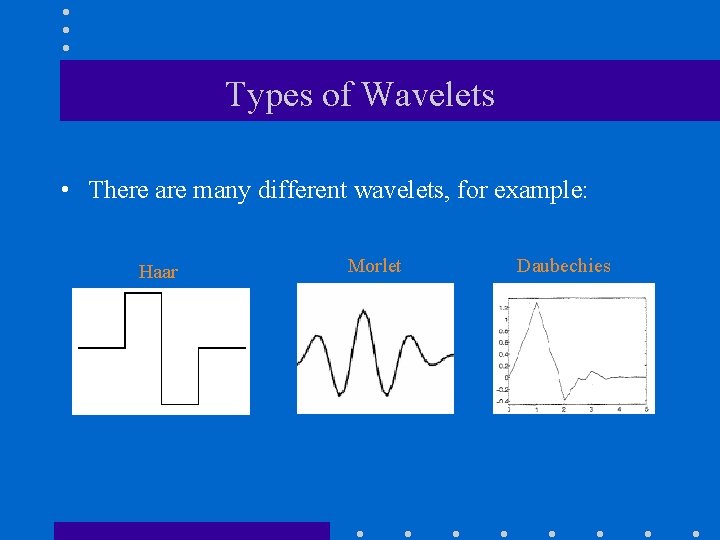
Types of Wavelets • There are many different wavelets, for example: Haar Morlet Daubechies

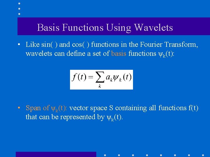
Basis Functions Using Wavelets • Like sin( ) and cos( ) functions in the Fourier Transform, wavelets can define a set of basis functions ψk(t): • Span of ψk(t): vector space S containing all functions f(t) that can be represented by ψk(t).

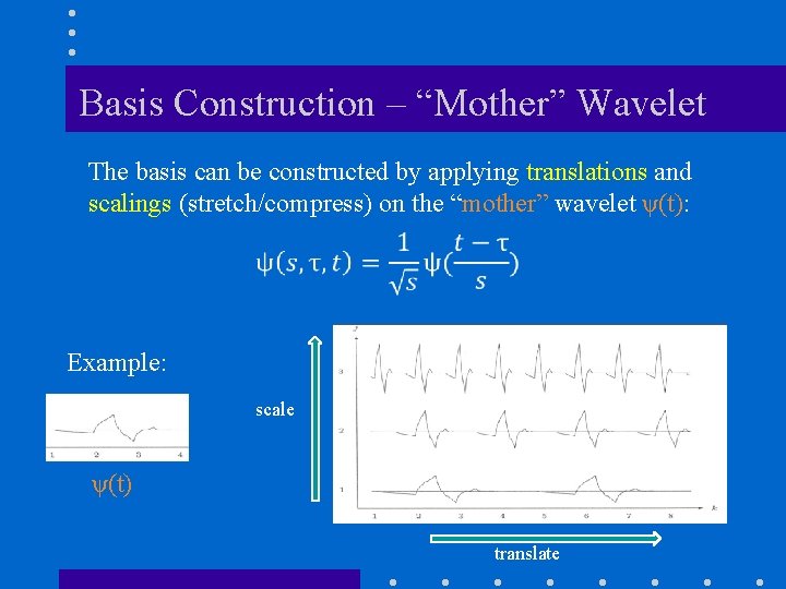
Basis Construction – “Mother” Wavelet The basis can be constructed by applying translations and scalings (stretch/compress) on the “mother” wavelet ψ(t): Example: scale ψ(t) translate

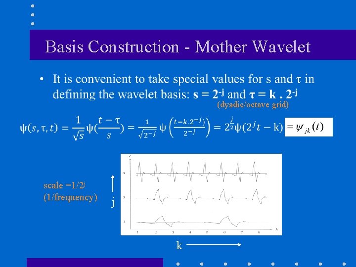
Basis Construction - Mother Wavelet (dyadic/octave grid) scale =1/2 j (1/frequency) j k

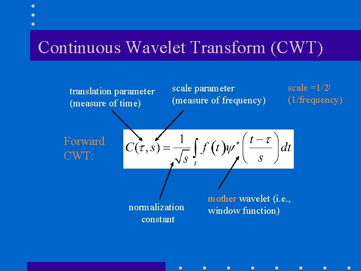
Continuous Wavelet Transform (CWT) translation parameter (measure of time) scale parameter (measure of frequency) scale =1/2 j (1/frequency) Forward CWT: normalization constant mother wavelet (i. e. , window function)

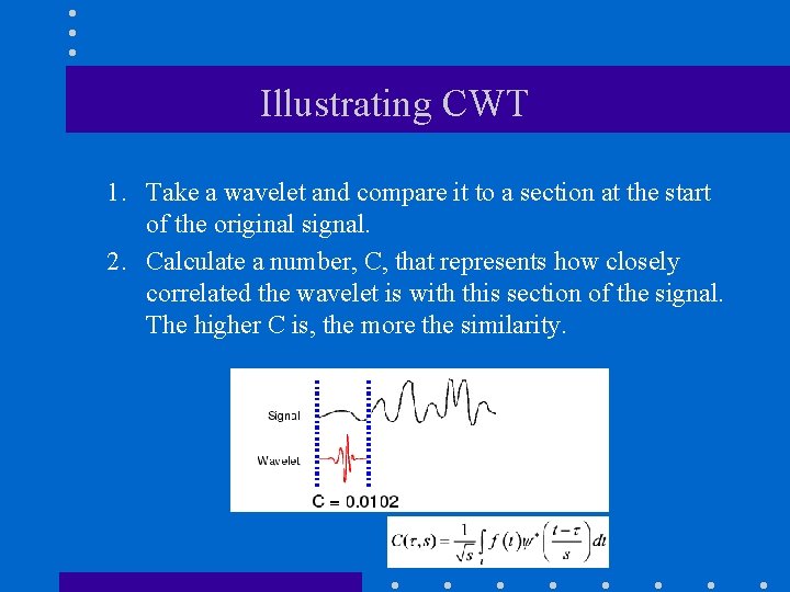
Illustrating CWT 1. Take a wavelet and compare it to a section at the start of the original signal. 2. Calculate a number, C, that represents how closely correlated the wavelet is with this section of the signal. The higher C is, the more the similarity.

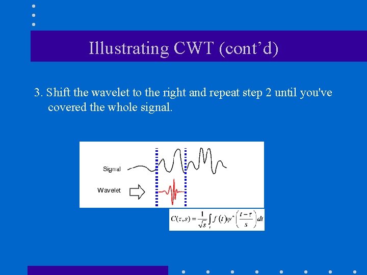
Illustrating CWT (cont’d) 3. Shift the wavelet to the right and repeat step 2 until you've covered the whole signal.

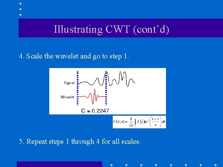
Illustrating CWT (cont’d) 4. Scale the wavelet and go to step 1. 5. Repeat steps 1 through 4 for all scales.

Visualize CTW Transform • Wavelet analysis produces a time-scale view of the input signal or image.

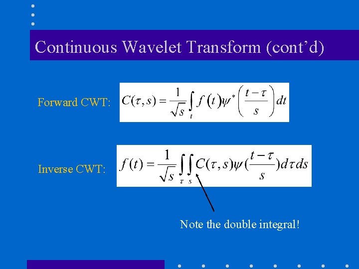
Continuous Wavelet Transform (cont’d) Forward CWT: Inverse CWT: Note the double integral!

Fourier Transform vs Wavelet Transform weighted by F(u)

Fourier Transform vs Wavelet Transform weighted by C(τ, s)

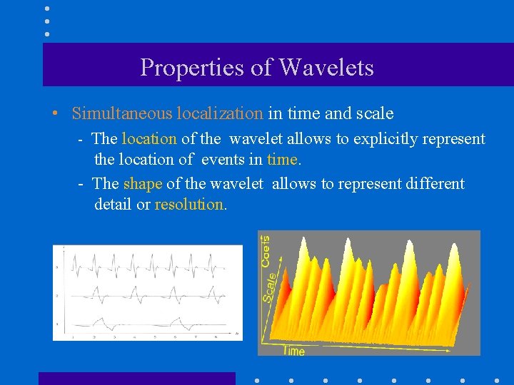
Properties of Wavelets • Simultaneous localization in time and scale - The location of the wavelet allows to explicitly represent the location of events in time. - The shape of the wavelet allows to represent different detail or resolution.

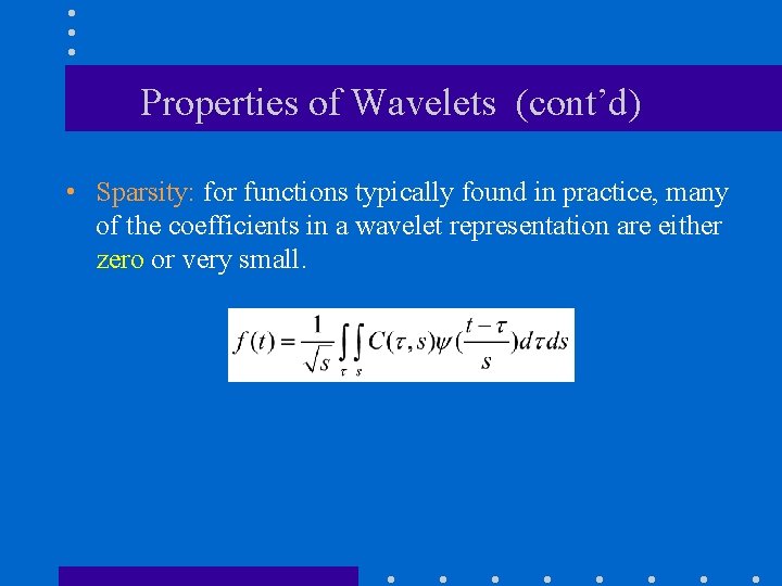
Properties of Wavelets (cont’d) • Sparsity: for functions typically found in practice, many of the coefficients in a wavelet representation are either zero or very small.

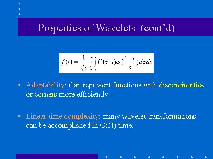
Properties of Wavelets (cont’d) • Adaptability: Can represent functions with discontinuities or corners more efficiently. • Linear-time complexity: many wavelet transformations can be accomplished in O(N) time.

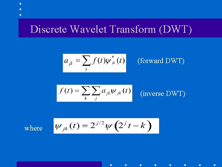
Discrete Wavelet Transform (DWT) (forward DWT) (inverse DWT) where

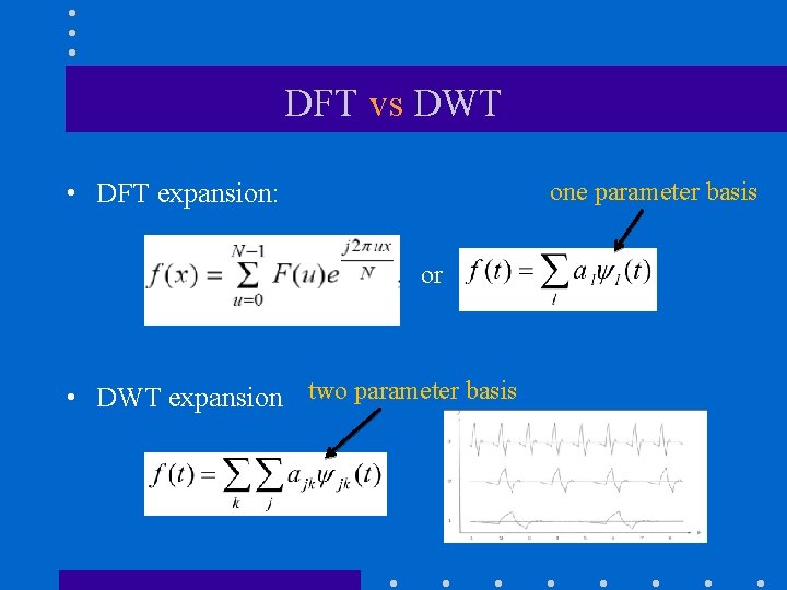
DFT vs DWT • DFT expansion: one parameter basis or • DWT expansion two parameter basis

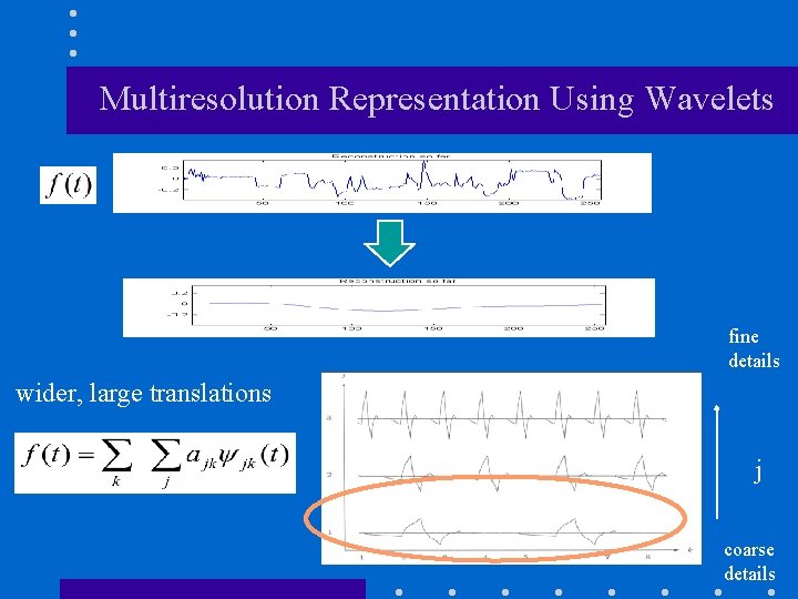
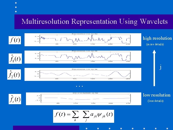
Multiresolution Representation Using Wavelets fine details wider, large translations j coarse details

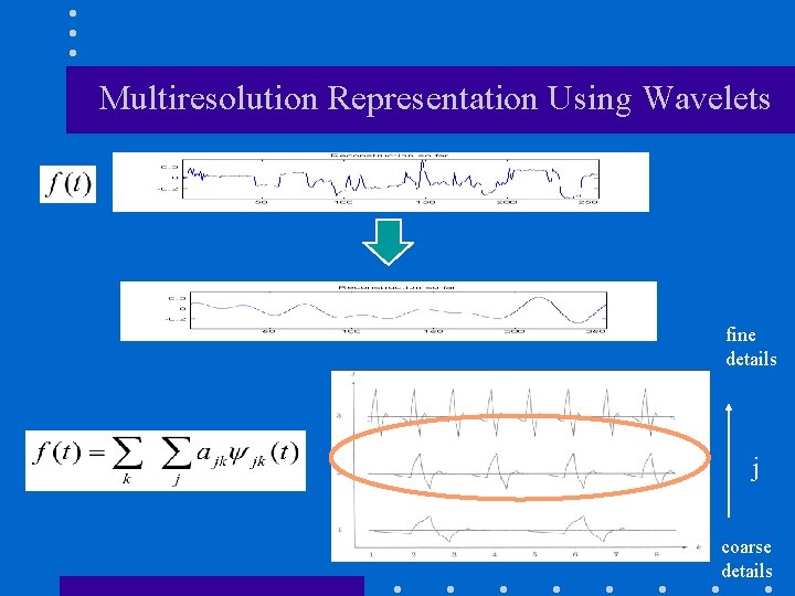
Multiresolution Representation Using Wavelets fine details j coarse details

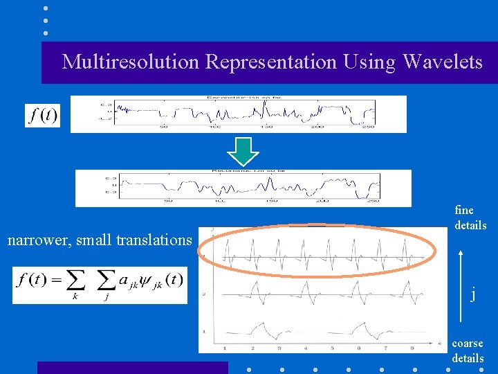
Multiresolution Representation Using Wavelets narrower, small translations fine details j coarse details

Multiresolution Representation Using Wavelets high resolution (more details) j … low resolution (less details)

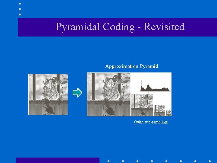
Pyramidal Coding - Revisited Approximation Pyramid (with sub-sampling)

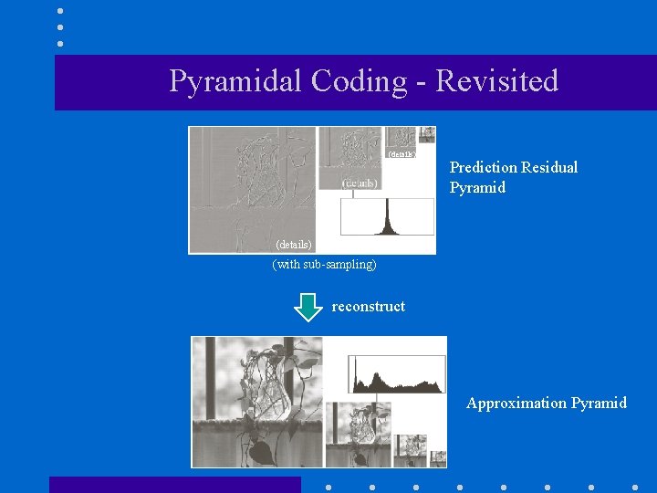
Pyramidal Coding - Revisited (details) Prediction Residual Pyramid (details) (with sub-sampling) reconstruct Approximation Pyramid

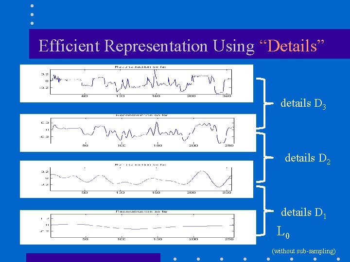
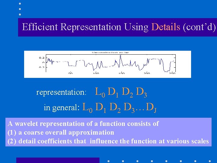
Efficient Representation Using “Details” details D 3 details D 2 details D 1 L 0 (without sub-sampling)

Efficient Representation Using Details (cont’d) L 0 D 1 D 2 D 3 in general: L 0 D 1 D 2 D 3…DJ representation: A wavelet representation of a function consists of (1) a coarse overall approximation (2) detail coefficients that influence the function at various scales

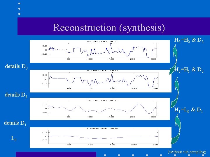
Reconstruction (synthesis) H 3=H 2 & D 3 details D 3 H 2=H 1 & D 2 details D 2 H 1=L 0 & D 1 details D 1 L 0 (without sub-sampling)

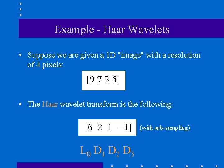
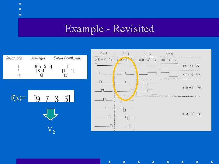
Example - Haar Wavelets • Suppose we are given a 1 D "image" with a resolution of 4 pixels: [9 7 3 5] • The Haar wavelet transform is the following: (with sub-sampling) L 0 D 1 D 2 D 3

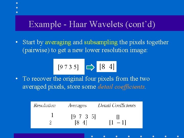
Example - Haar Wavelets (cont’d) • Start by averaging and subsampling the pixels together (pairwise) to get a new lower resolution image: [9 7 3 5] • To recover the original four pixels from the two averaged pixels, store some detail coefficients. 1

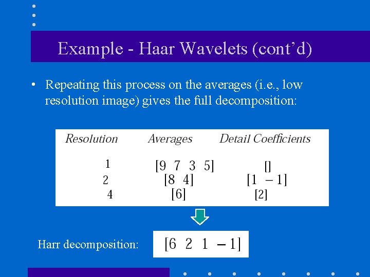
Example - Haar Wavelets (cont’d) • Repeating this process on the averages (i. e. , low resolution image) gives the full decomposition: 1 Harr decomposition:

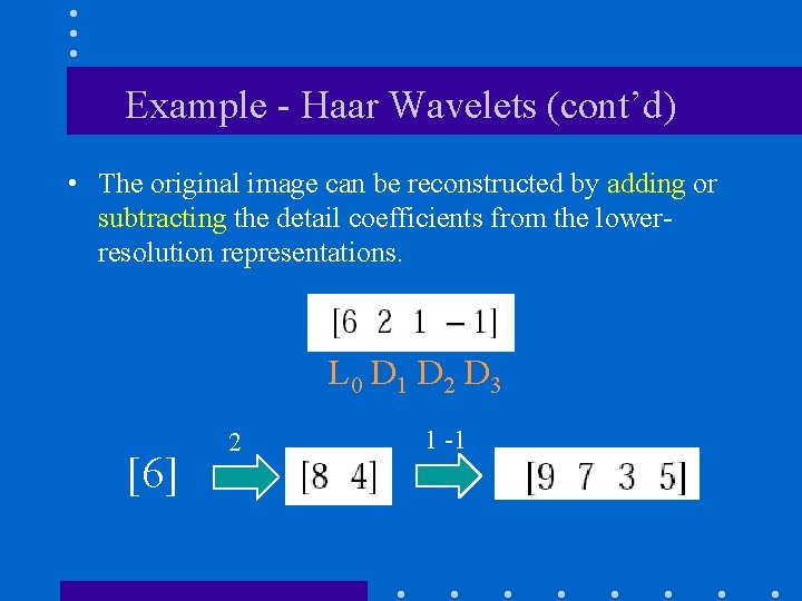
Example - Haar Wavelets (cont’d) • The original image can be reconstructed by adding or subtracting the detail coefficients from the lowerresolution representations. L 0 D 1 D 2 D 3 [6] 2 1 -1

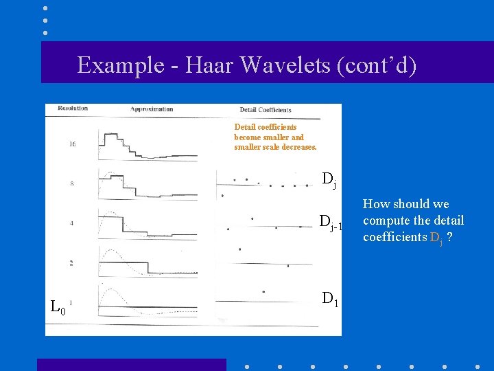
Example - Haar Wavelets (cont’d) Detail coefficients become smaller and smaller scale decreases. Dj Dj-1 L 0 D 1 How should we compute the detail coefficients Dj ?

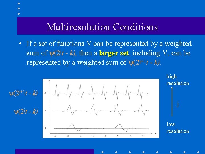
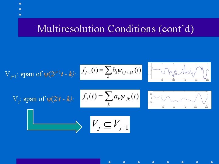
Multiresolution Conditions • If a set of functions V can be represented by a weighted sum of ψ(2 jt - k), then a larger set, set including V, can be represented by a weighted sum of ψ(2 j+1 t - k). high resolution ψ(2 j+1 t - k) j ψ(2 jt - k) low resolution

Multiresolution Conditions (cont’d) Vj+1: span of ψ(2 j+1 t - k): Vj: span of ψ(2 jt - k):

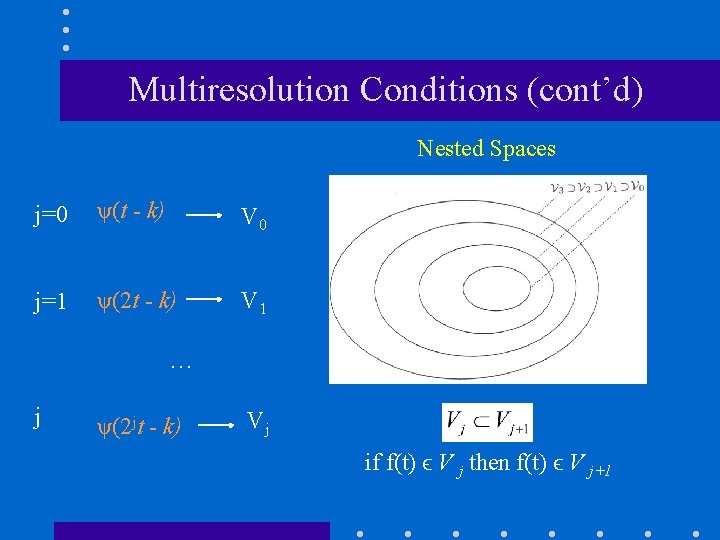
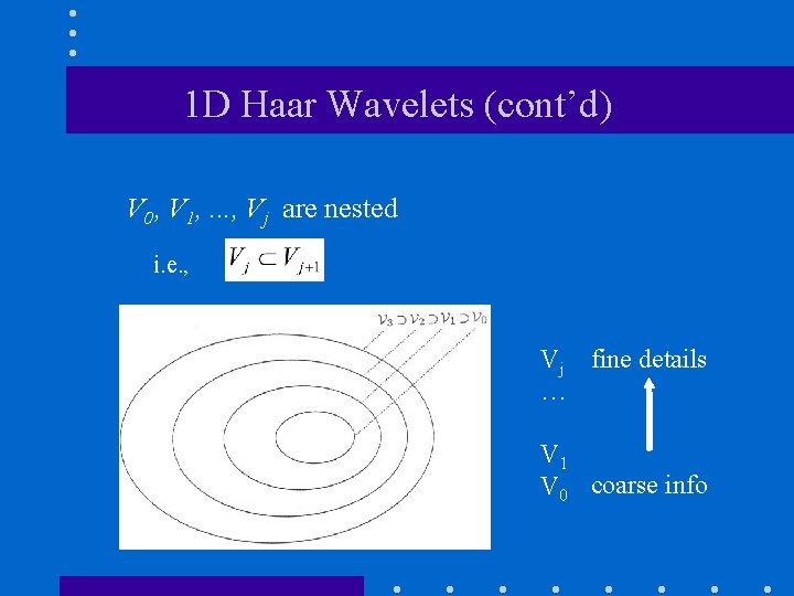
Multiresolution Conditions (cont’d) Nested Spaces j=0 ψ(t - k) V 0 j=1 ψ(2 t - k) V 1 … j ψ(2 jt - k) Vj if f(t) ϵ V j then f(t) ϵ V j+1

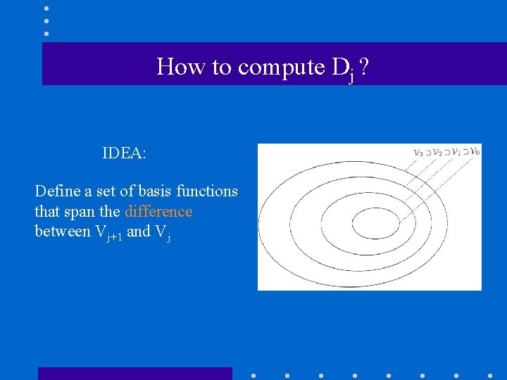
How to compute Dj ? IDEA: Define a set of basis functions that span the difference between Vj+1 and Vj

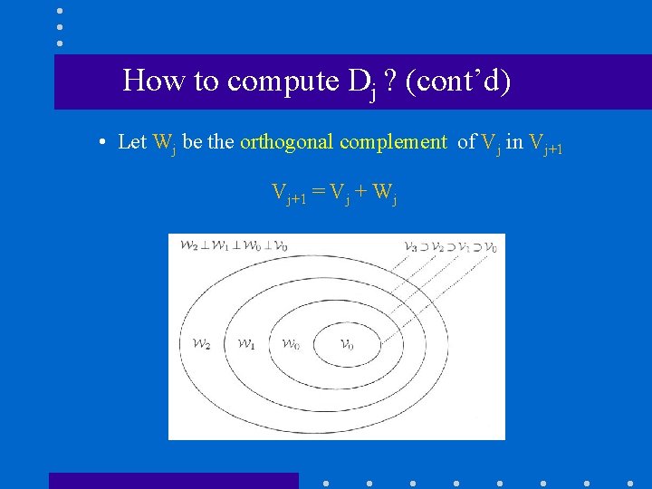
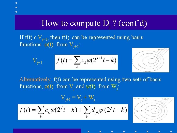
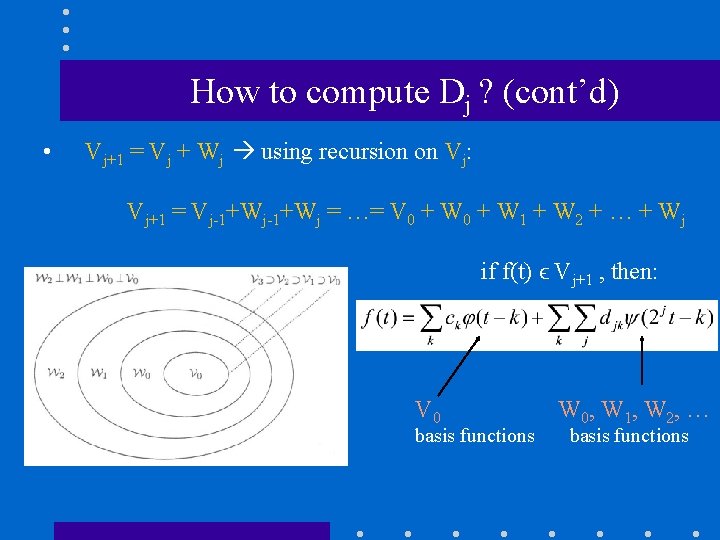
How to compute Dj ? (cont’d) • Let Wj be the orthogonal complement of Vj in Vj+1 = Vj + Wj

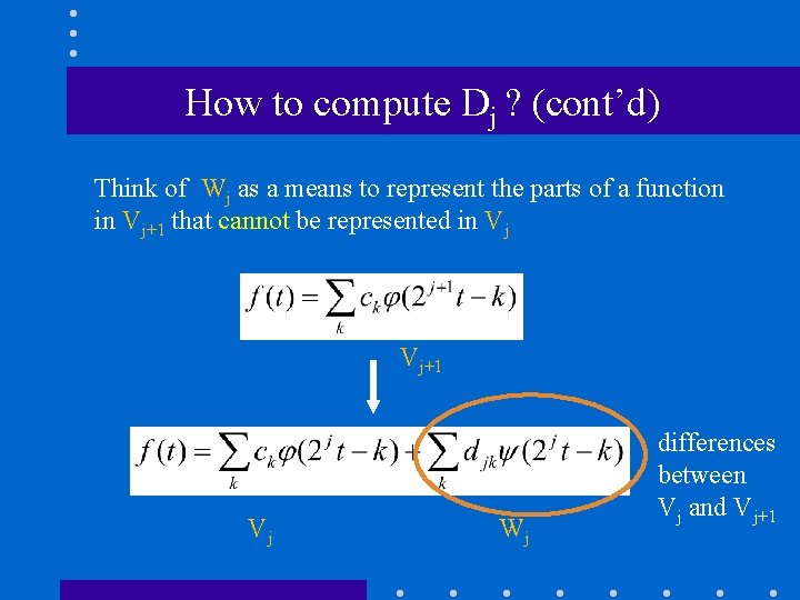
How to compute Dj ? (cont’d) If f(t) ϵ Vj+1, then f(t) can be represented using basis functions φ(t) from Vj+1: Vj+1 Alternatively, f(t) can be represented using two sets of basis functions, φ(t) from Vj and ψ(t) from Wj: Vj+1 = Vj + Wj

How to compute Dj ? (cont’d) Think of Wj as a means to represent the parts of a function in Vj+1 that cannot be represented in Vj Vj+1 Vj Wj differences between Vj and Vj+1

How to compute Dj ? (cont’d) • Vj+1 = Vj + Wj using recursion on Vj: Vj+1 = Vj-1+Wj = …= V 0 + W 1 + W 2 + … + Wj if f(t) ϵ Vj+1 , then: V 0 basis functions W 0, W 1, W 2, … basis functions

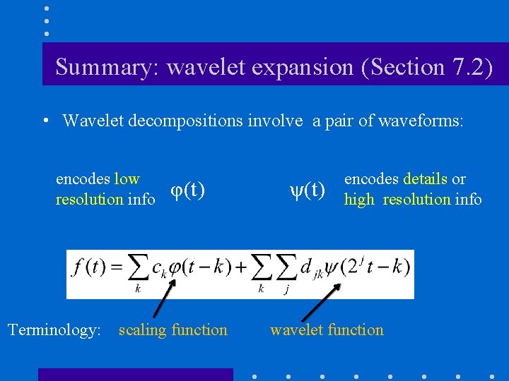
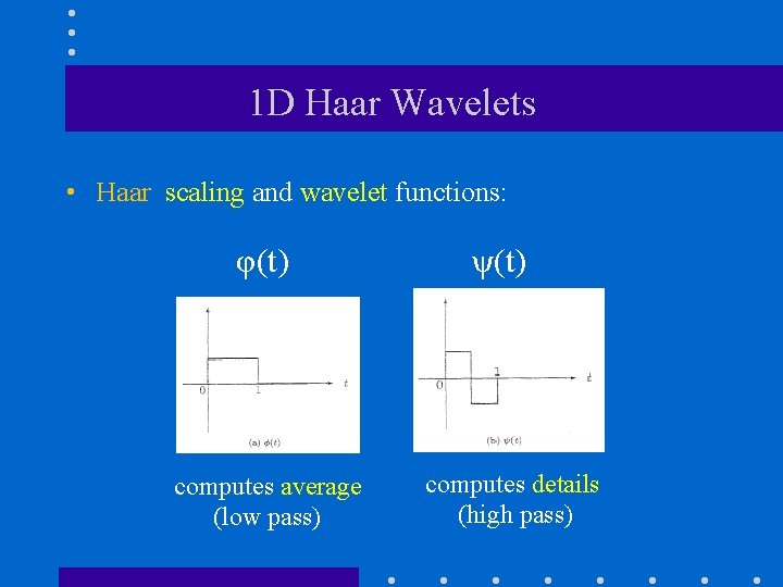
Summary: wavelet expansion (Section 7. 2) • Wavelet decompositions involve a pair of waveforms: encodes low resolution info Terminology: φ(t) scaling function ψ(t) encodes details or high resolution info wavelet function

1 D Haar Wavelets • Haar scaling and wavelet functions: φ(t) computes average (low pass) ψ(t) computes details (high pass)

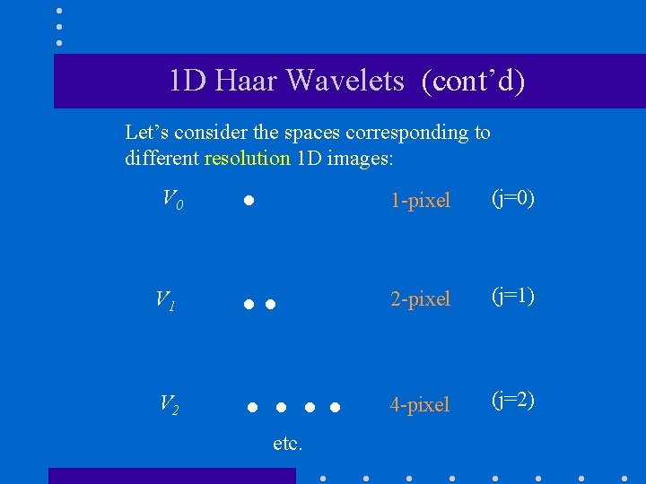
1 D Haar Wavelets (cont’d) Let’s consider the spaces corresponding to different resolution 1 D images: V 0 V 1 V 2 . . . …. etc. 1 -pixel (j=0) 2 -pixel (j=1) 4 -pixel (j=2)

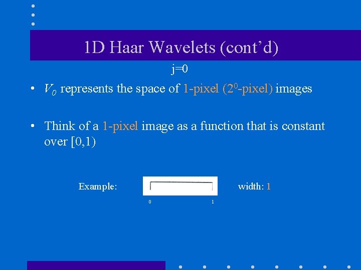
1 D Haar Wavelets (cont’d) j=0 • V 0 represents the space of 1 -pixel (20 -pixel) images • Think of a 1 -pixel image as a function that is constant over [0, 1) Example: width: 1 0 1

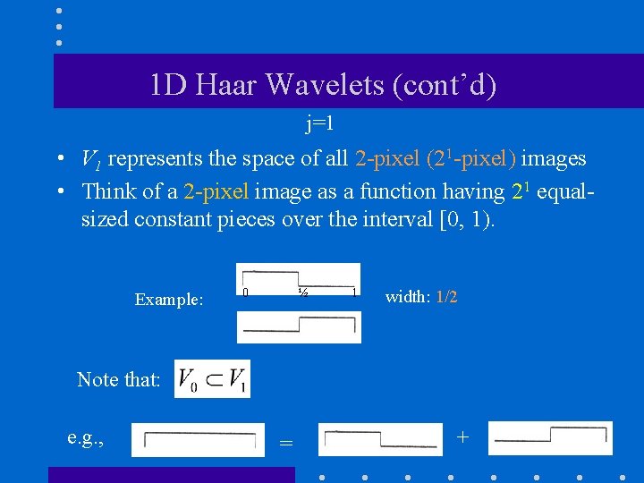
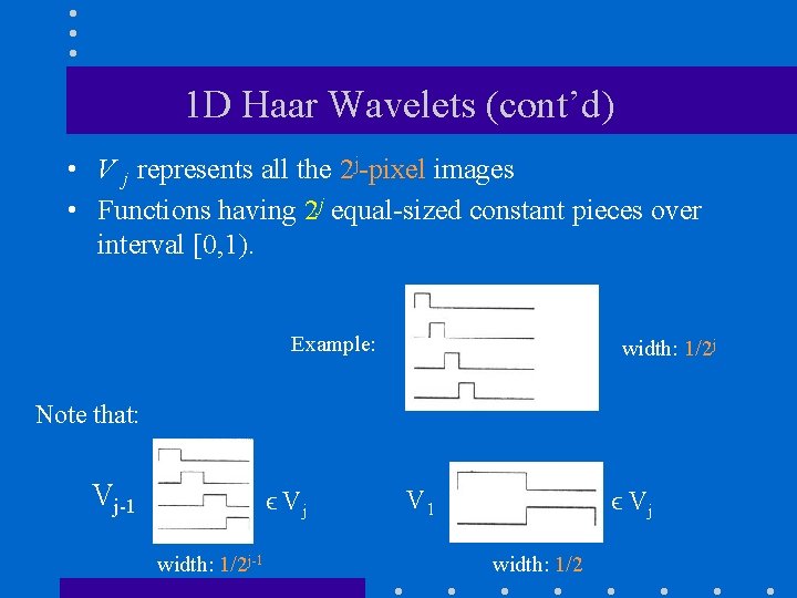
1 D Haar Wavelets (cont’d) j=1 • V 1 represents the space of all 2 -pixel (21 -pixel) images • Think of a 2 -pixel image as a function having 21 equalsized constant pieces over the interval [0, 1). Example: 0 ½ 1 width: 1/2 Note that: e. g. , = +

1 D Haar Wavelets (cont’d) • V j represents all the 2 j-pixel images • Functions having 2 j equal-sized constant pieces over interval [0, 1). Example: width: 1/2 j Note that: Vj-1 ϵ Vj width: 1/2 j-1 V 1 ϵ Vj width: 1/2

1 D Haar Wavelets (cont’d) V 0, V 1, . . . , Vj are nested i. e. , Vj fine details … V 1 V 0 coarse info

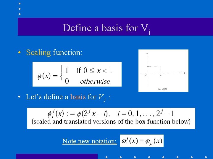
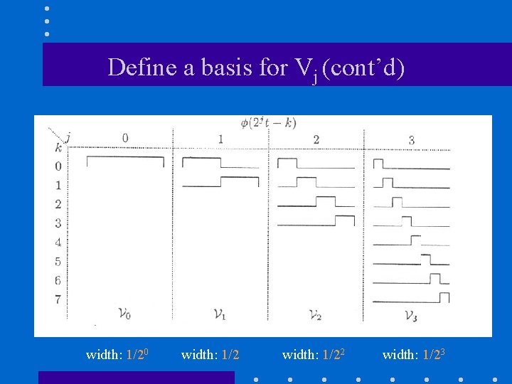
Define a basis for Vj • Scaling function: • Let’s define a basis for V j : Note new notation:

Define a basis for Vj (cont’d) width: 1/20 width: 1/22 width: 1/23

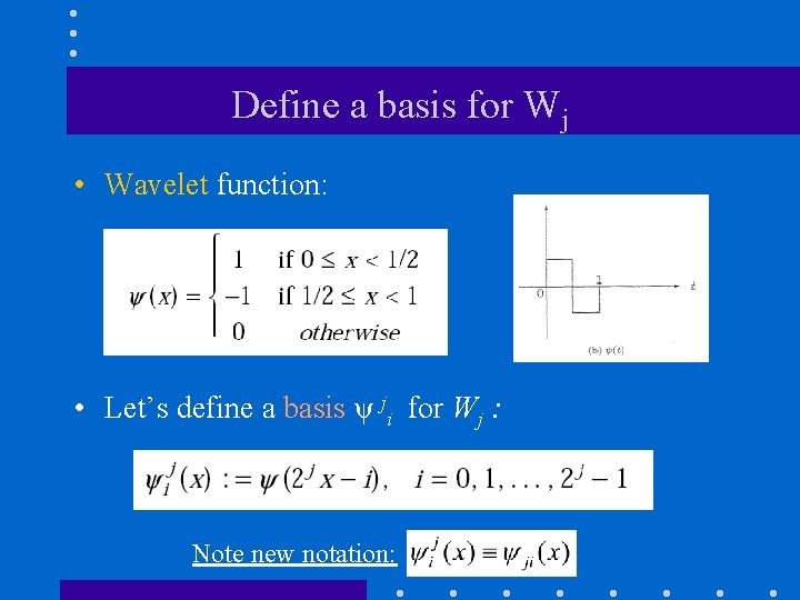
Define a basis for Wj • Wavelet function: • Let’s define a basis ψ ji for Wj : Note new notation:

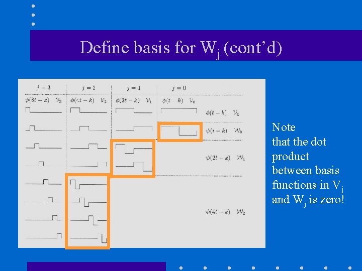
Define basis for Wj (cont’d) Note that the dot product between basis functions in Vj and Wj is zero!

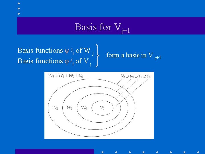
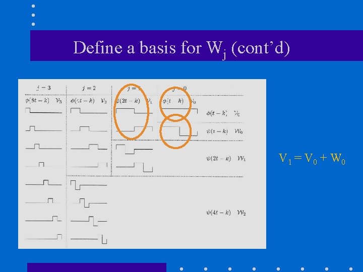
Basis for Vj+1 Basis functions ψ ji of W j Basis functions φ ji of V j form a basis in V j+1

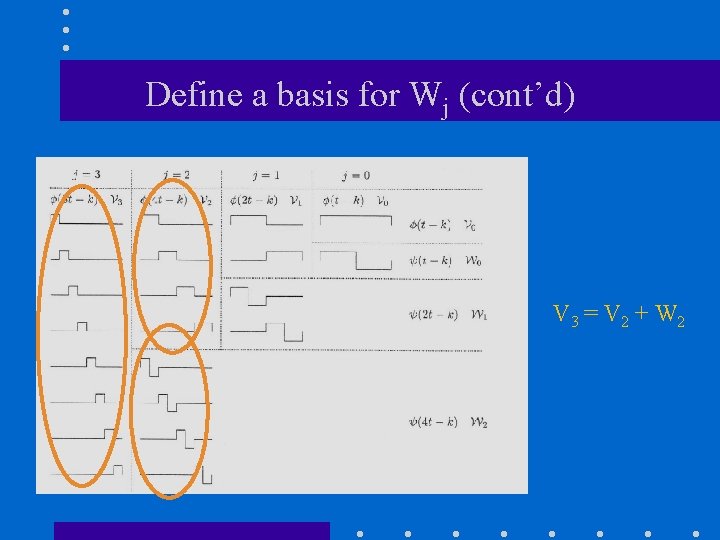
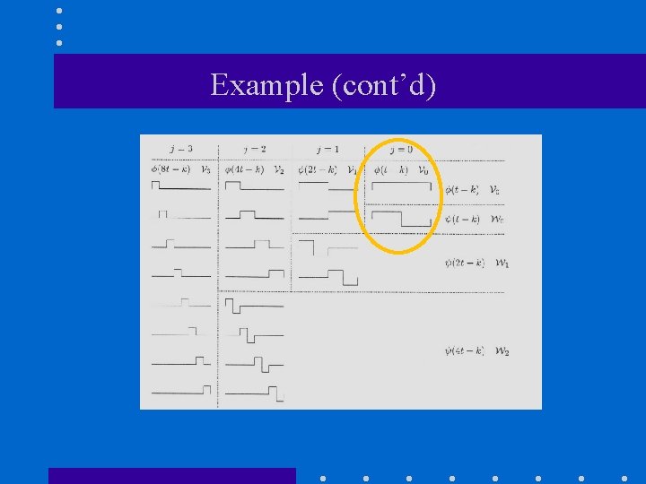
Define a basis for Wj (cont’d) V 3 = V 2 + W 2

Define a basis for Wj (cont’d) V 2 = V 1 + W 1

Define a basis for Wj (cont’d) V 1 = V 0 + W 0

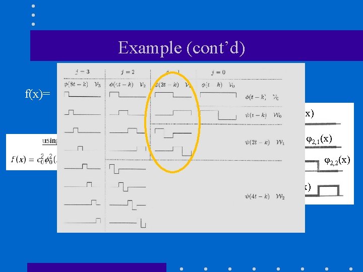
Example - Revisited f(x)= V 2

Example (cont’d) f(x)= φ2, 0(x) V 2 φ2, 1(x) φ2, 2(x) φ2, 3(x)

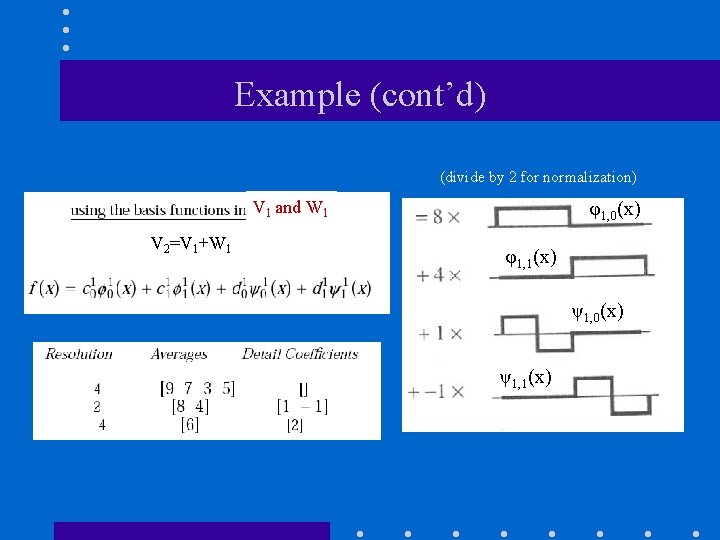
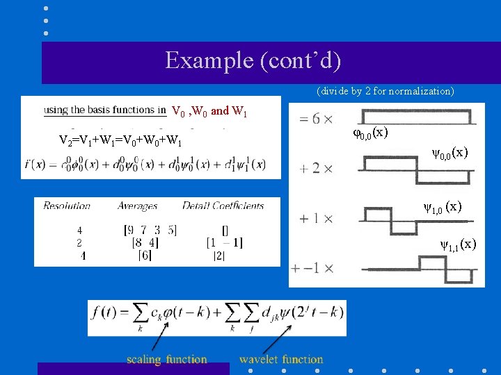
Example (cont’d) (divide by 2 for normalization) V 1 and W 1 V 2=V 1+W 1 φ1, 0(x) φ1, 1(x) ψ1, 0(x) ψ1, 1(x)

Example (cont’d)

Example (cont’d) (divide by 2 for normalization) V 0 , W 0 and W 1 V 2=V 1+W 1=V 0+W 1 φ0, 0(x) ψ1, 0 (x) ψ1, 1(x)

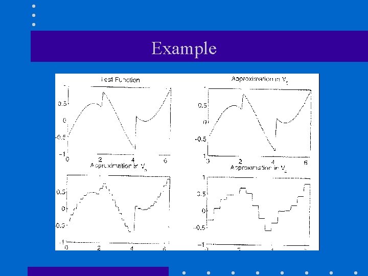
Example

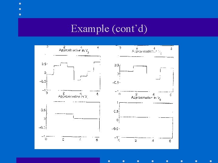
Example (cont’d)

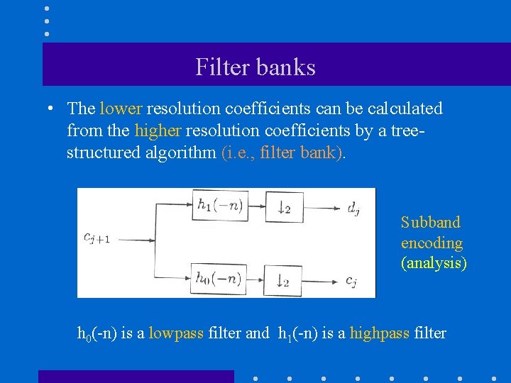
Filter banks • The lower resolution coefficients can be calculated from the higher resolution coefficients by a treestructured algorithm (i. e. , filter bank). Subband encoding (analysis) h 0(-n) is a lowpass filter and h 1(-n) is a highpass filter

Example (revisited) [9 7 3 5] low-pass, down-sampling (9+7)/2 high-pass, down-sampling (3+5)/2 (9 -7)/2 (3 -5)/2 LP HP

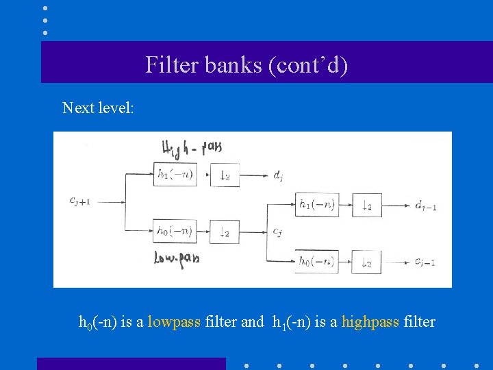
Filter banks (cont’d) Next level: h 0(-n) is a lowpass filter and h 1(-n) is a highpass filter

Example (revisited) [9 7 3 5] low-pass, down-sampling high-pass, down-sampling LP (8+4)/2 (8 -4)/2 HP

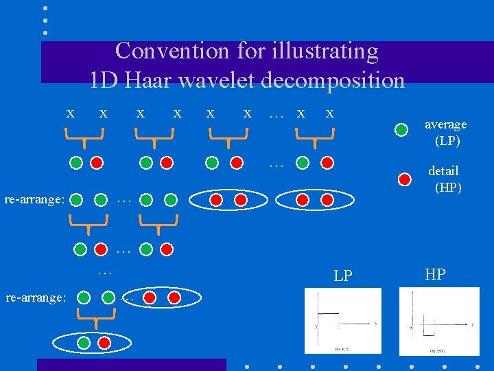
Convention for illustrating 1 D Haar wavelet decomposition x x x … detail (HP) … re-arrange: average (LP) … … re-arrange: LP … HP

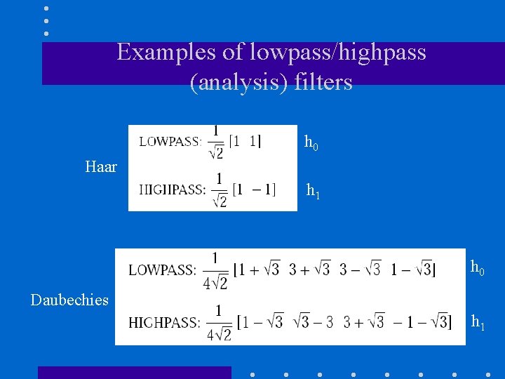
Examples of lowpass/highpass (analysis) filters h 0 Haar h 1 h 0 Daubechies h 1

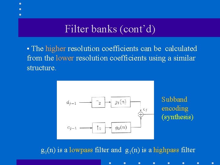
Filter banks (cont’d) • The higher resolution coefficients can be calculated from the lower resolution coefficients using a similar structure. Subband encoding (synthesis) g 0(n) is a lowpass filter and g 1(n) is a highpass filter

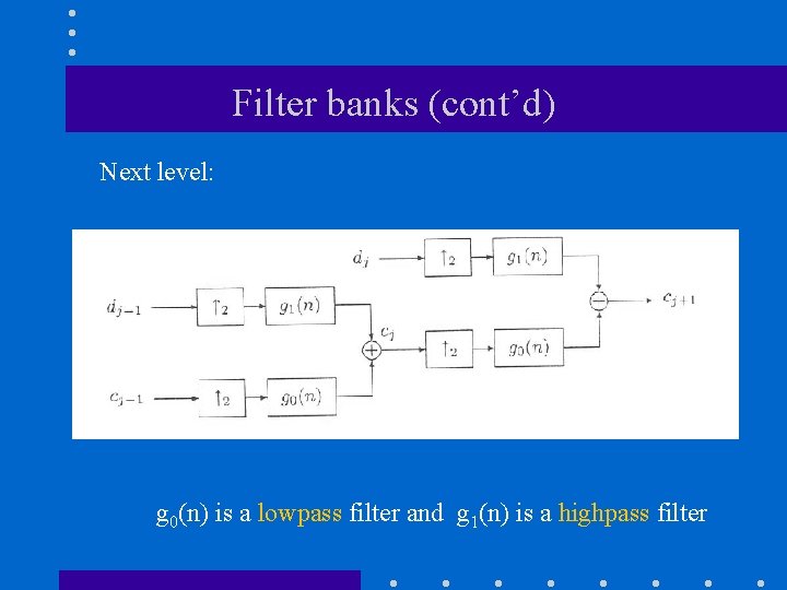
Filter banks (cont’d) Next level: g 0(n) is a lowpass filter and g 1(n) is a highpass filter

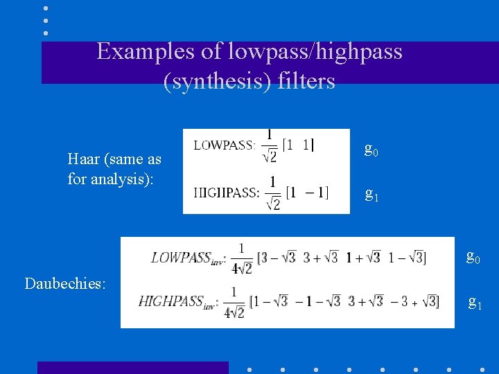
Examples of lowpass/highpass (synthesis) filters Haar (same as for analysis): g 0 g 1 g 0 Daubechies: + g 1

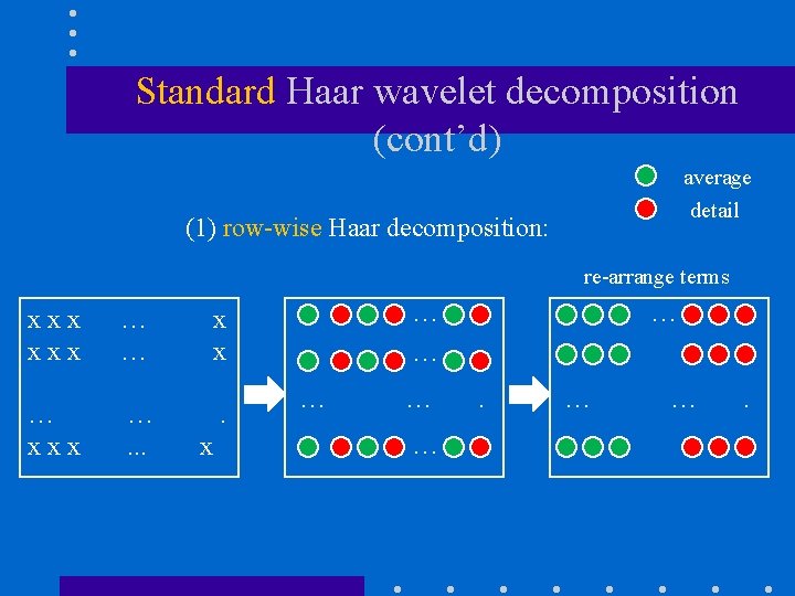
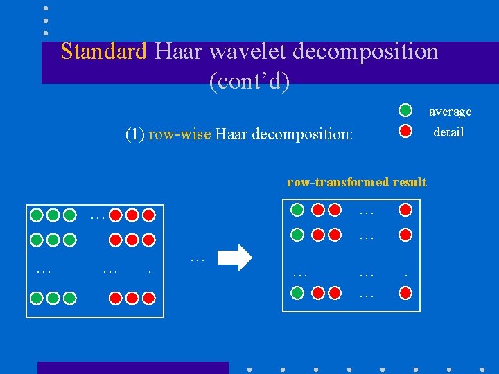
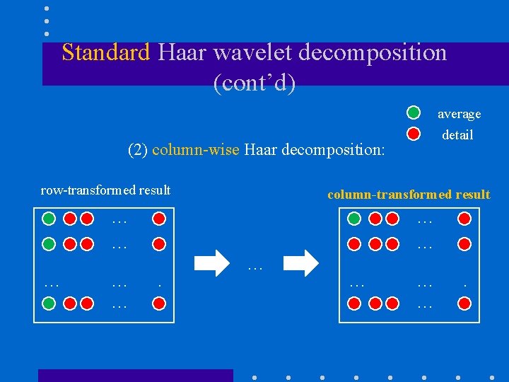
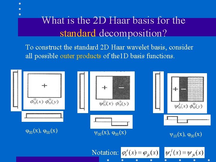
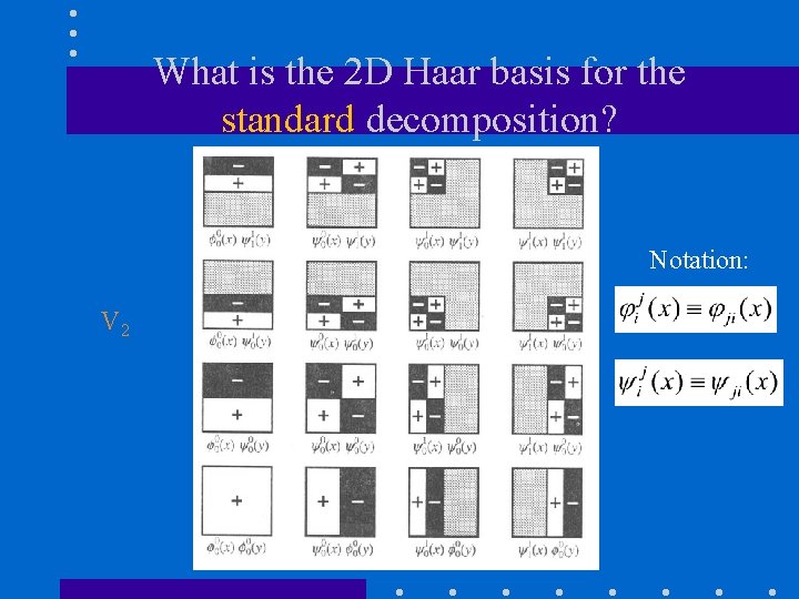
2 D Haar Wavelet Transform • The 2 D Haar wavelet decomposition can be computed using 1 D Haar wavelet decompositions. – i. e. , 2 D Haar wavelet basis is separable • We’ll discuss two different decompositions (i. e. , correspond to different basis functions): – Standard decomposition – Non-standard decomposition

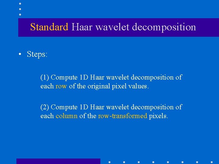
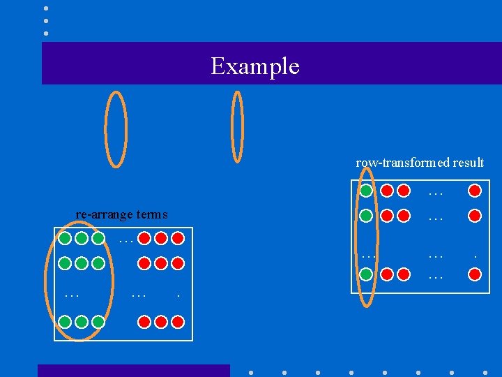
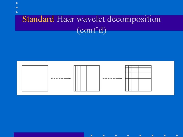
Standard Haar wavelet decomposition • Steps: (1) Compute 1 D Haar wavelet decomposition of each row of the original pixel values. (2) Compute 1 D Haar wavelet decomposition of each column of the row-transformed pixels.

Standard Haar wavelet decomposition (cont’d) average detail (1) row-wise Haar decomposition: re-arrange terms xxx … … x x … xxx …. . x … … … .

Standard Haar wavelet decomposition (cont’d) average detail (1) row-wise Haar decomposition: row-transformed result … … … .

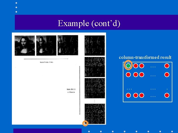
Standard Haar wavelet decomposition (cont’d) average detail (2) column-wise Haar decomposition: row-transformed result column-transformed result … … … … .

Example row-transformed result … … re-arrange terms … … .

Example (cont’d) column-transformed result … … … .

Standard Haar wavelet decomposition (cont’d)

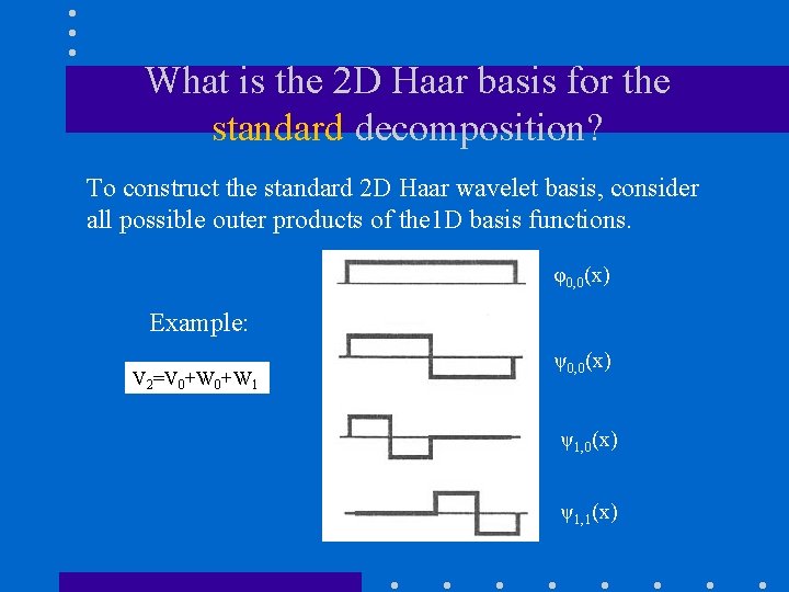
What is the 2 D Haar basis for the standard decomposition? To construct the standard 2 D Haar wavelet basis, consider all possible outer products of the 1 D basis functions. φ0, 0(x) Example: V 2=V 0+W 1 ψ0, 0(x) ψ1, 1(x)

What is the 2 D Haar basis for the standard decomposition? To construct the standard 2 D Haar wavelet basis, consider all possible outer products of the 1 D basis functions. φ00(x), φ00(x) ψ00(x), φ00(x) Notation: ψ10(x), φ00(x)

What is the 2 D Haar basis for the standard decomposition? Notation: V 2

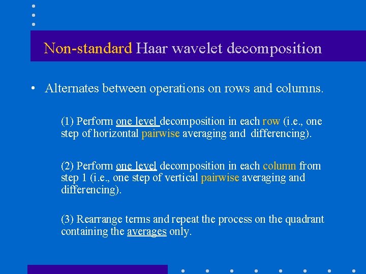
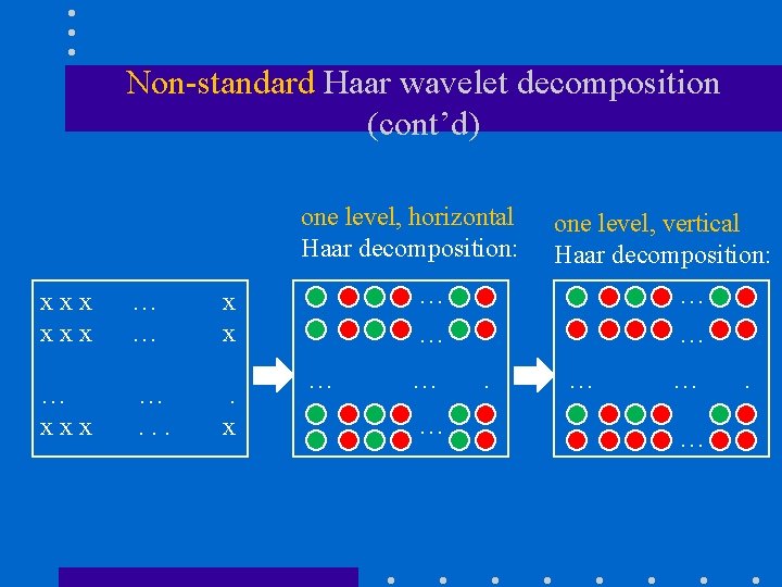
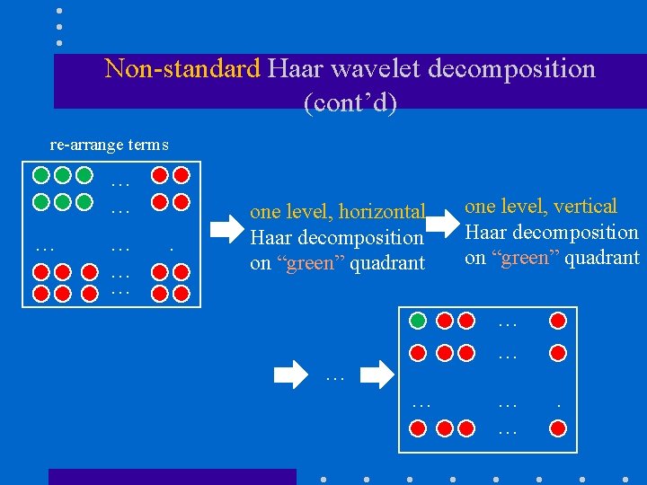
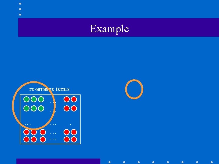
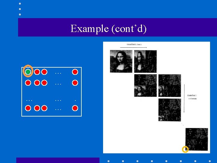
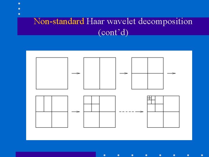
Non-standard Haar wavelet decomposition • Alternates between operations on rows and columns. (1) Perform one level decomposition in each row (i. e. , one step of horizontal pairwise averaging and differencing). (2) Perform one level decomposition in each column from step 1 (i. e. , one step of vertical pairwise averaging and differencing). (3) Rearrange terms and repeat the process on the quadrant containing the averages only.

Non-standard Haar wavelet decomposition (cont’d) one level, horizontal Haar decomposition: xxx … … x x … xxx …. . x one level, vertical Haar decomposition: … … … … .

Non-standard Haar wavelet decomposition (cont’d) re-arrange terms … … … . one level, horizontal Haar decomposition on “green” quadrant one level, vertical Haar decomposition on “green” quadrant … … … .

Example re-arrange terms … … … .

Example (cont’d) … … … .

Non-standard Haar wavelet decomposition (cont’d)

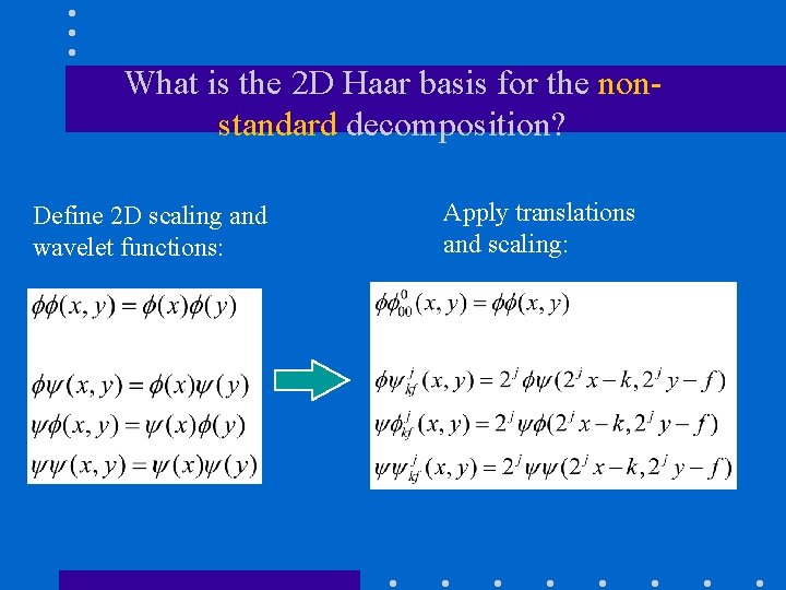
What is the 2 D Haar basis for the nonstandard decomposition? Define 2 D scaling and wavelet functions: Apply translations and scaling:

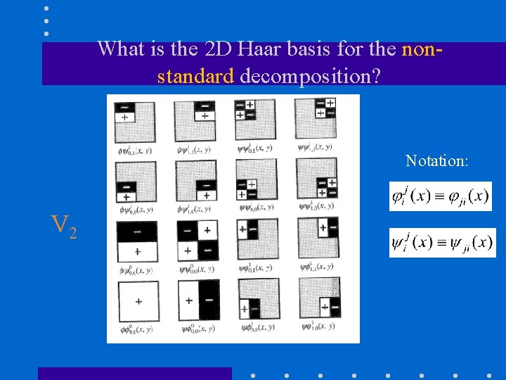
What is the 2 D Haar basis for the nonstandard decomposition? Notation: V 2

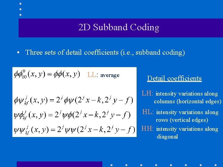
2 D Subband Coding • Three sets of detail coefficients (i. e. , subband coding) LL: average LL Detail coefficients LH: intensity variations along columns (horizontal edges) HL: intensity variations along HH: rows (vertical edges) intensity variations along diagonal

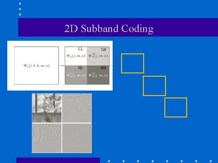
2 D Subband Coding LL LH HL HH

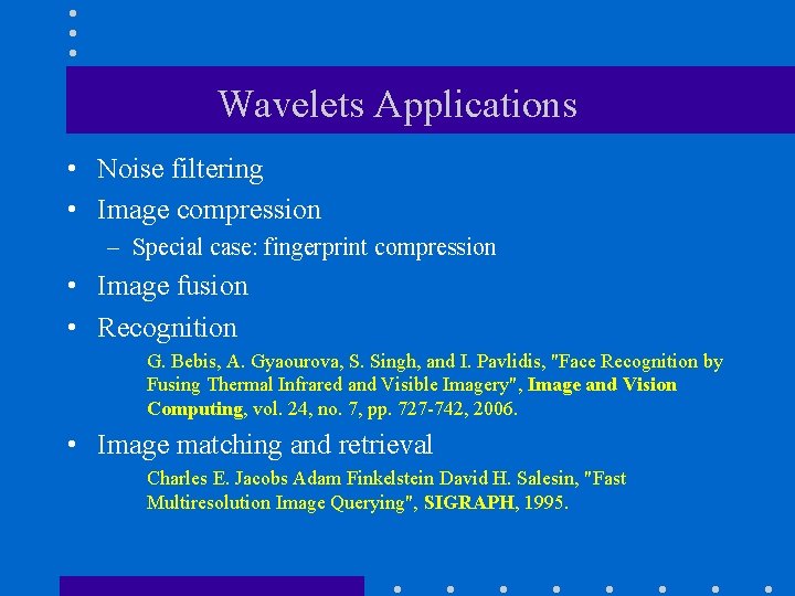
Wavelets Applications • Noise filtering • Image compression – Special case: fingerprint compression • Image fusion • Recognition G. Bebis, A. Gyaourova, S. Singh, and I. Pavlidis, "Face Recognition by Fusing Thermal Infrared and Visible Imagery", Image and Vision Computing, vol. 24, no. 7, pp. 727 -742, 2006. • Image matching and retrieval Charles E. Jacobs Adam Finkelstein David H. Salesin, "Fast Multiresolution Image Querying", SIGRAPH, 1995.