Digital Image Processing Lecture 6 Image Geometry January

Digital Image Processing Lecture 6: Image Geometry January 13, 2004 Prof. Charlene Tsai Digital Image Processing Lecture 6

Before Lecture … § Homework 2 is out online (due date: 3/28). Digital Image Processing Lecture 6 2

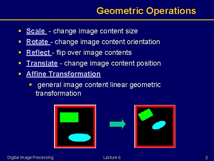
Geometric Operations § § § Scale - change image content size Rotate - change image content orientation Reflect - flip over image contents Translate - change image content position Affine Transformation § general image content linear geometric transformation Digital Image Processing Lecture 6 3

Geometric transformations § Geometric transformations are common in computer graphics, and are often used in image analysis. § Geometric transforms permit the elimination of geometric distortion that occurs when an image is captured. § If one attempts to match two different images of the same object, a geometric transformation may be needed. § Examples? Digital Image Processing Lecture 6 4

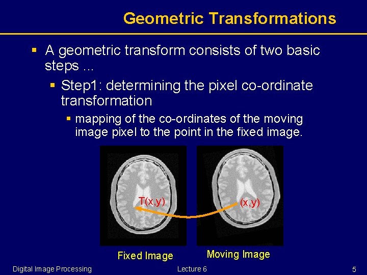
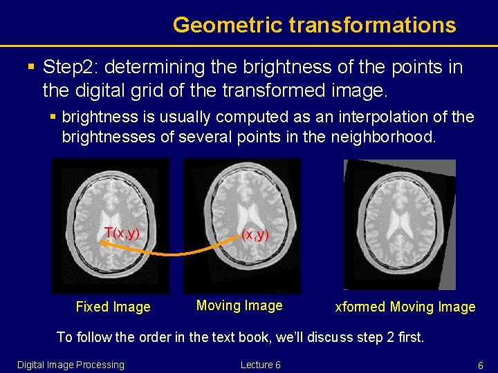
Geometric Transformations § A geometric transform consists of two basic steps. . . § Step 1: determining the pixel co-ordinate transformation § mapping of the co-ordinates of the moving image pixel to the point in the fixed image. T(x, y) Fixed Image Digital Image Processing (x, y) Moving Image Lecture 6 5

Geometric transformations § Step 2: determining the brightness of the points in the digital grid of the transformed image. § brightness is usually computed as an interpolation of the brightnesses of several points in the neighborhood. T(x, y) Fixed Image (x, y) Moving Image xformed Moving Image To follow the order in the text book, we’ll discuss step 2 first. Digital Image Processing Lecture 6 6

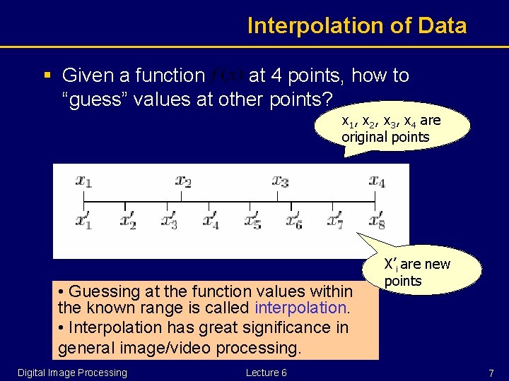
Interpolation of Data § Given a function at 4 points, how to “guess” values at other points? x 1, x 2, x 3, x 4 are original points • Guessing at the function values within the known range is called interpolation. • Interpolation has great significance in general image/video processing. Digital Image Processing Lecture 6 X’i are new points 7

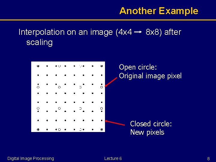
Another Example Interpolation on an image (4 x 4 scaling 8 x 8) after Open circle: Original image pixel Closed circle: New pixels Digital Image Processing Lecture 6 8

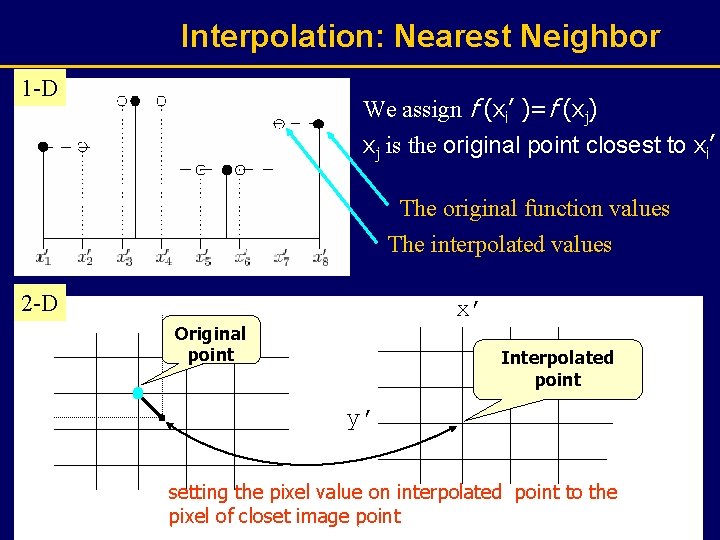
Interpolation: Nearest Neighbor 1 -D We assign f (xi’ )=f (xj) xj is the original point closest to xi’ The original function values The interpolated values 2 -D x’ Original point Interpolated point y’ setting the pixel value on interpolated point to the pixel of closet image point Digital Image Processing Lecture 6 9

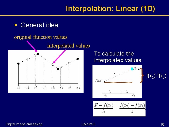
Interpolation: Linear (1 D) § General idea: original function values interpolated values To calculate the interpolated values f(x 2)-f(x 1) Digital Image Processing Lecture 6 10

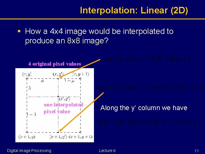
Interpolation: Linear (2 D) § How a 4 x 4 image would be interpolated to produce an 8 x 8 image? 4 original pixel values one interpolated pixel value Digital Image Processing Along the y’ column we have Lecture 6 11

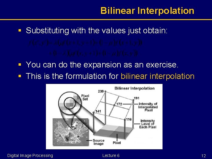
Bilinear Interpolation § Substituting with the values just obtain: § You can do the expansion as an exercise. § This is the formulation for bilinear interpolation Digital Image Processing Lecture 6 12

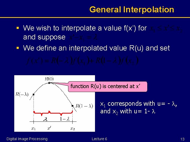
General Interpolation § We wish to interpolate a value f(x’) for and suppose § We define an interpolated value R(u) and set function R(u) is centered at x’ x 1 corresponds with u= - , and x 2 with u= 1 - Digital Image Processing Lecture 6 13

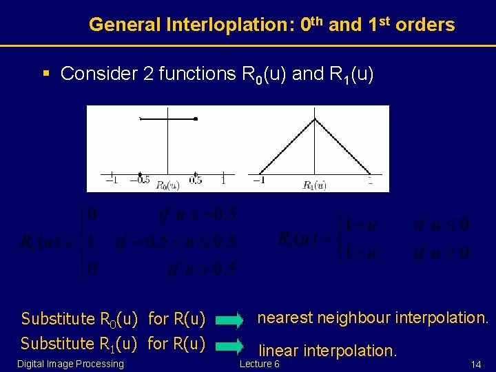
General Interloplation: 0 th and 1 st orders § Consider 2 functions R 0(u) and R 1(u) Substitute R 0(u) for R(u) Substitute R 1(u) for R(u) Digital Image Processing nearest neighbour interpolation. linear interpolation. Lecture 6 14

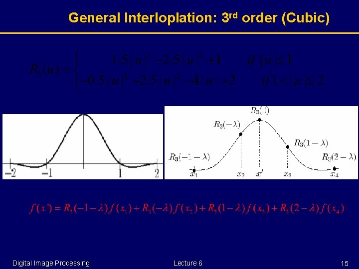
General Interloplation: 3 rd order (Cubic) Digital Image Processing Lecture 6 15

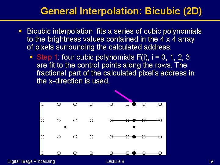
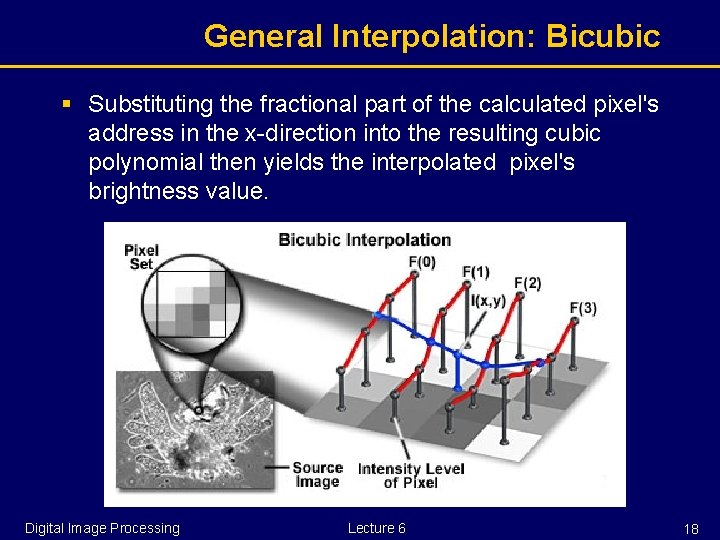
General Interpolation: Bicubic (2 D) § Bicubic interpolation fits a series of cubic polynomials to the brightness values contained in the 4 x 4 array of pixels surrounding the calculated address. § Step 1: four cubic polynomials F(i), i = 0, 1, 2, 3 are fit to the control points along the rows. The fractional part of the calculated pixel's address in the x-direction is used. Digital Image Processing Lecture 6 16

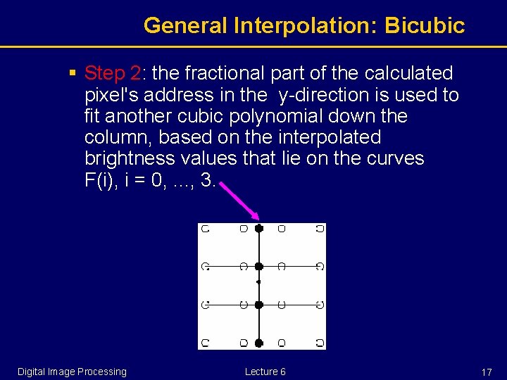
General Interpolation: Bicubic § Step 2: the fractional part of the calculated pixel's address in the y-direction is used to fit another cubic polynomial down the column, based on the interpolated brightness values that lie on the curves F(i), i = 0, . . . , 3. Digital Image Processing Lecture 6 17

General Interpolation: Bicubic § Substituting the fractional part of the calculated pixel's address in the x-direction into the resulting cubic polynomial then yields the interpolated pixel's brightness value. Digital Image Processing Lecture 6 18

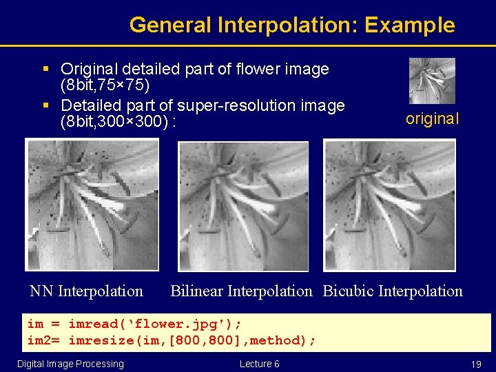
General Interpolation: Example § Original detailed part of flower image (8 bit, 75× 75) § Detailed part of super-resolution image (8 bit, 300× 300) : NN Interpolation original Bilinear Interpolation Bicubic Interpolation im = imread(‘flower. jpg'); im 2= imresize(im, [800, 800], method); Digital Image Processing Lecture 6 19

General Interpolation: Summary § For NN interpolation, the output pixel is assigned the value of the pixel that the point falls within. No other pixels are considered. § For bilinear interpolation, the output pixel value is a weighted average of pixels in the nearest 2 -by-2 neighborhood. § For bicubic interpolation, the output pixel value is a weighted average of pixels in the nearest 4 -by-4 neighborhood. § Bilinear method takes longer than nearest neighbor interpolation, and the bicubic method takes longer than bilinear. § The greater the number of pixels considered, the more accurate the computation is, so there is a tradeoff between processing time and quality. Digital Image Processing Lecture 6 20

Scaling Operation § To shrink or zoom the size of an image (or part of an image). § To change the visual appearance of an image; § To alter the quantity of information § To use as a low-level pre-processor in multistage image processing chain which operates on features of a particular scale. § Scaling is a special case of affine transformation. § The matlab command is simply “imresize”. Digital Image Processing Lecture 6 21

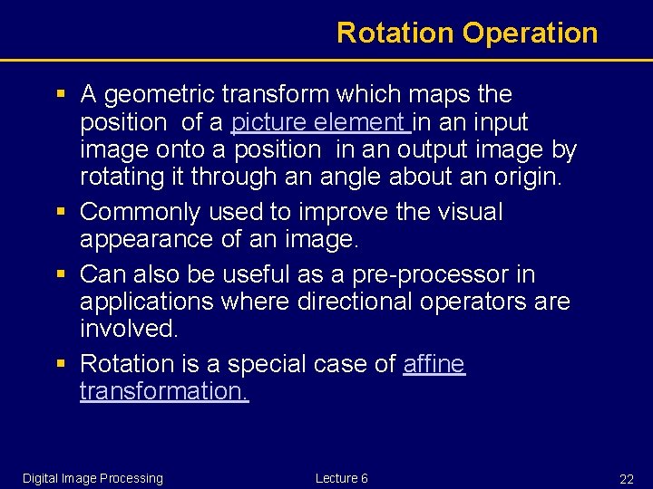
Rotation Operation § A geometric transform which maps the position of a picture element in an input image onto a position in an output image by rotating it through an angle about an origin. § Commonly used to improve the visual appearance of an image. § Can also be useful as a pre-processor in applications where directional operators are involved. § Rotation is a special case of affine transformation. Digital Image Processing Lecture 6 22

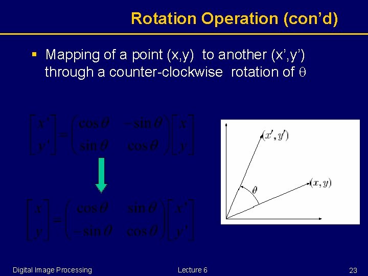
Rotation Operation (con’d) § Mapping of a point (x, y) to another (x’, y’) through a counter-clockwise rotation of Digital Image Processing Lecture 6 23

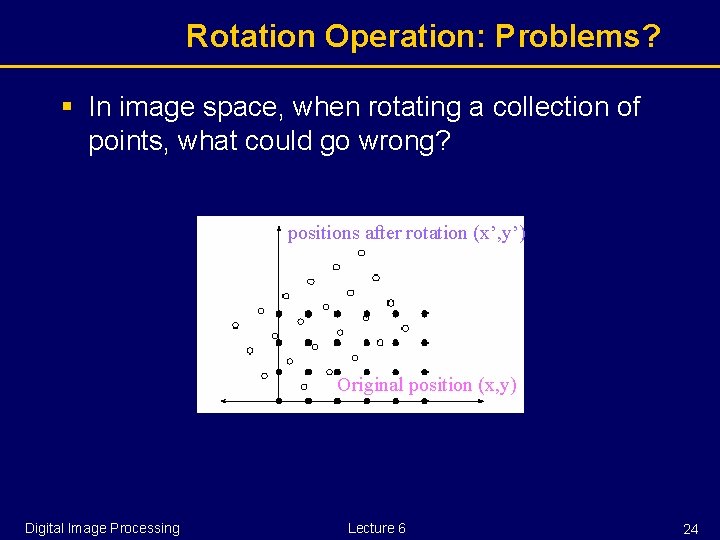
Rotation Operation: Problems? § In image space, when rotating a collection of points, what could go wrong? positions after rotation (x’, y’) Original position (x, y) Digital Image Processing Lecture 6 24

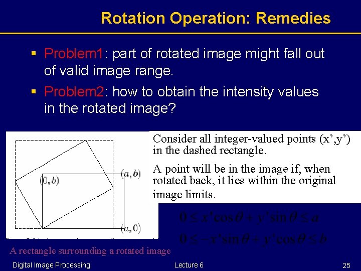
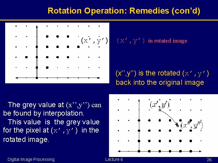
Rotation Operation: Remedies § Problem 1: part of rotated image might fall out of valid image range. § Problem 2: how to obtain the intensity values in the rotated image? Consider all integer-valued points (x’, y’) in the dashed rectangle. A point will be in the image if, when rotated back, it lies within the original image limits. A rectangle surrounding a rotated image Digital Image Processing Lecture 6 25

Rotation Operation: Remedies (con’d) (x’, y’) in rotated image (x’’, y’’) is the rotated (x’, y’) back into the original image • The grey value at (x’’, y’’) can be found by interpolation. • This value is the grey value for the pixel at (x’, y’) in the rotated image. Digital Image Processing Lecture 6 26

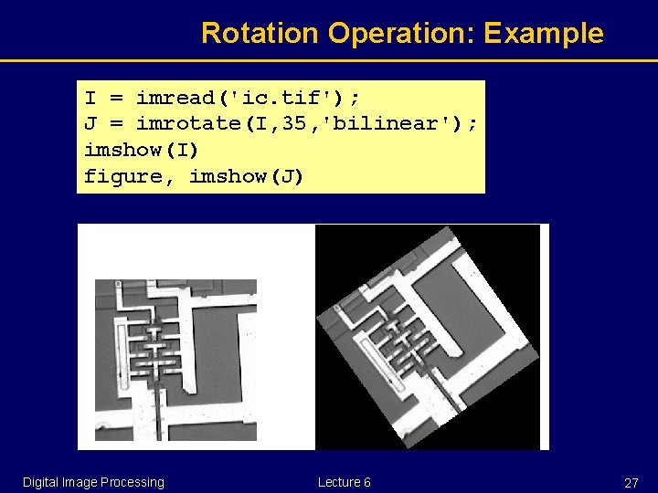
Rotation Operation: Example I = imread('ic. tif'); J = imrotate(I, 35, 'bilinear'); imshow(I) figure, imshow(J) Digital Image Processing Lecture 6 27

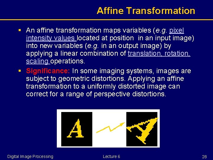
Affine Transformation § An affine transformation maps variables (e. g. pixel intensity values located at position in an input image) into new variables (e. g. in an output image) by applying a linear combination of translation, rotation, scaling operations. § Significance: In some imaging systems, images are subject to geometric distortions. Applying an affine transformation to a uniformly distorted image can correct for a range of perspective distortions. Digital Image Processing Lecture 6 28

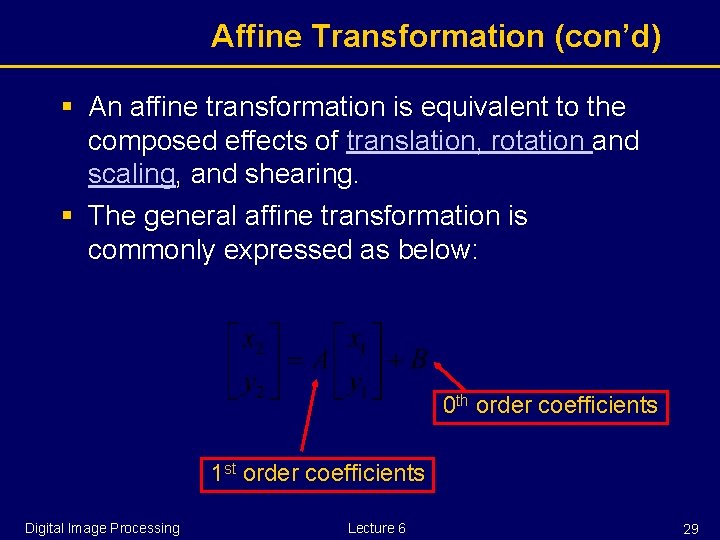
Affine Transformation (con’d) § An affine transformation is equivalent to the composed effects of translation, rotation and scaling, and shearing. § The general affine transformation is commonly expressed as below: 0 th order coefficients 1 st order coefficients Digital Image Processing Lecture 6 29

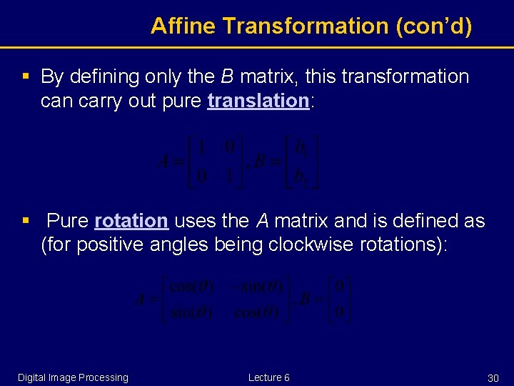
Affine Transformation (con’d) § By defining only the B matrix, this transformation carry out pure translation: § Pure rotation uses the A matrix and is defined as (for positive angles being clockwise rotations): Digital Image Processing Lecture 6 30

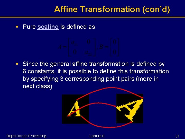
Affine Transformation (con’d) § Pure scaling is defined as § Since the general affine transformation is defined by 6 constants, it is possible to define this transformation by specifying 3 corresponding point pairs (more in next class). Digital Image Processing Lecture 6 31

Matlab imtransform § The imtransform function accepts two primary arguments: § The image to be transformed § A spatial transformation structure, called a TFORM, that specifies the type of transformation you want to perform § Specify the type of transformation in a TFORM structure. Two ways to create a TFORM struct: § Using the maketform function § Using the cp 2 tform function Digital Image Processing Lecture 6 32

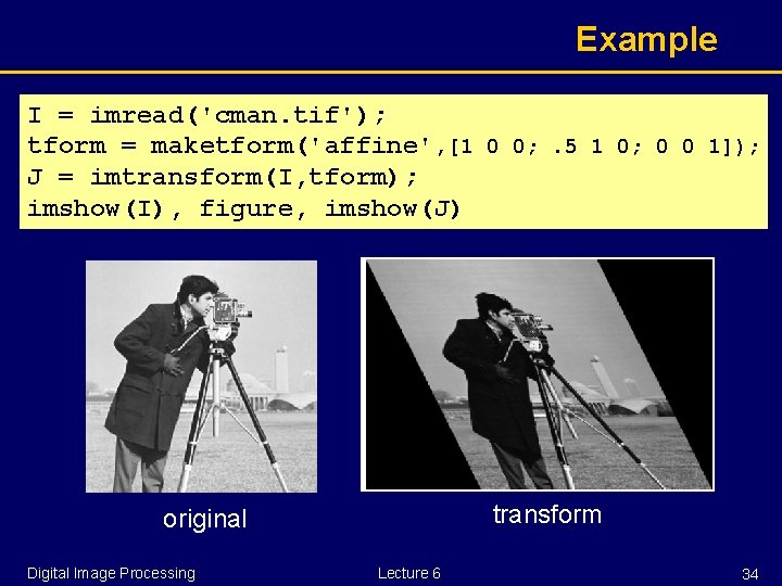
Using maketform § When using the maketform function, you can specify the type of transformation, e. g § § 'affine’ 'projective’ 'composite‘, et al ‘custom' and 'composite' capabilities of maketform allow a virtually limitless variety of spatial transformations to be used § Once you define the transformation in a TFORM struct, you canperform the transformation by calling imtransform. Digital Image Processing Lecture 6 33

Example I = imread('cman. tif'); tform = maketform('affine', [1 0 0; . 5 1 0; 0 0 1]); J = imtransform(I, tform); imshow(I), figure, imshow(J) transform original Digital Image Processing Lecture 6 34

Summary § Interpolation of intensity values on non-grid points: § Nearest Neibhgor (NN) § Bilinear § Bicubic § Image transformation § Computation of intensity values of the transformed image § Discussed some instances of affine transformation § Translation § Rotation § Scaling Digital Image Processing Lecture 6 35