Digital Image Processing Image Compression Lecture 2 Image

Digital Image Processing Image Compression Lecture 2

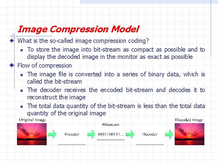
Image Compression Model What is the so-called image compression coding? n To store the image into bit-stream as compact as possible and to display the decoded image in the monitor as exact as possible Flow of compression n The image file is converted into a series of binary data, which is called the bit-stream n The decoder receives the encoded bit-stream and decodes it to reconstruct the image n The total data quantity of the bit-stream is less than the total data quantity of the original image

Fidelity Criteria The degree of exactness with which something is copied or reproduced The general classes of criteria : 1. Objective fidelity criteria 2. Subjective fidelity criteria H. R. Pourreza

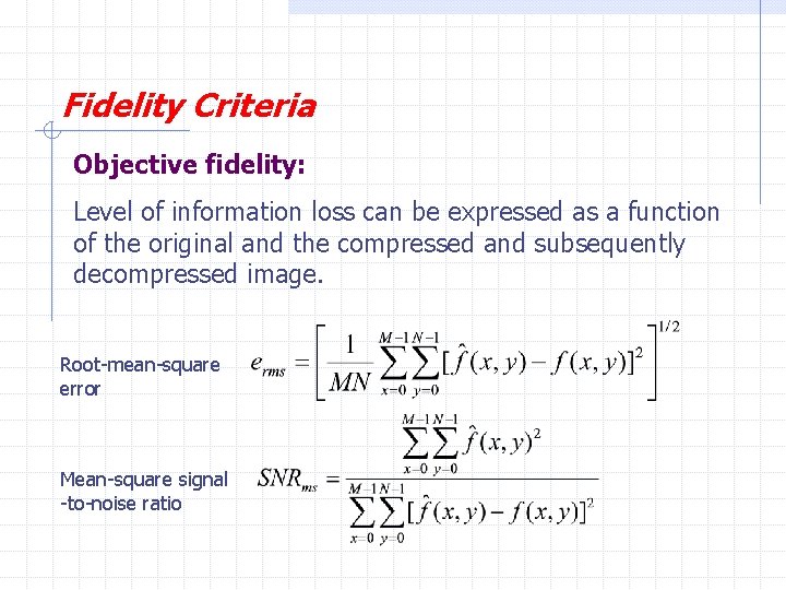
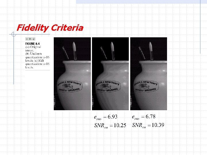
Fidelity Criteria Objective fidelity: Level of information loss can be expressed as a function of the original and the compressed and subsequently decompressed image. Root-mean-square error Mean-square signal -to-noise ratio

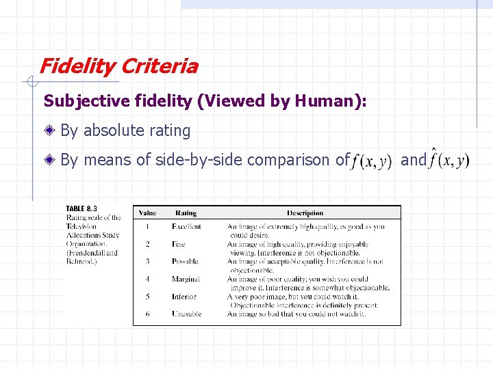
Fidelity Criteria Subjective fidelity (Viewed by Human): By absolute rating By means of side-by-side comparison of and

Fidelity Criteria

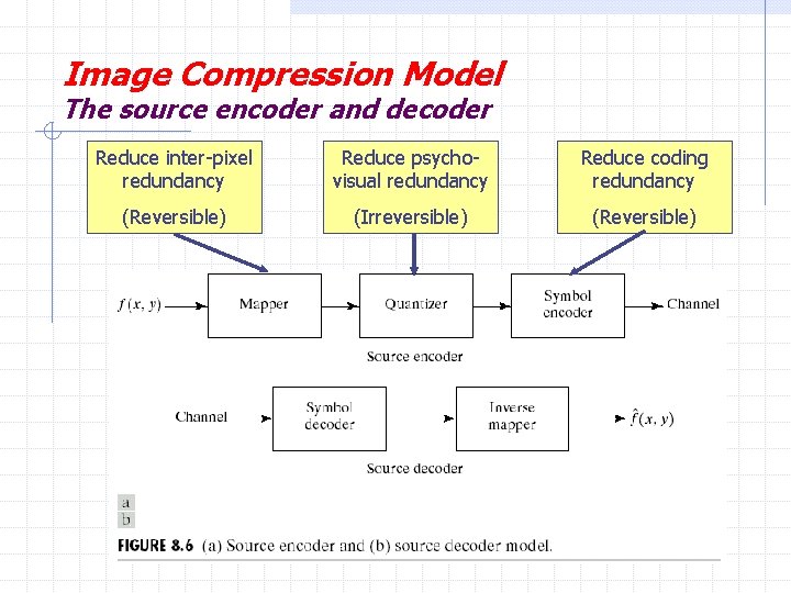
Image Compression Model The source encoder and decoder Reduce inter-pixel redundancy Reduce psychovisual redundancy Reduce coding redundancy (Reversible) (Irreversible) (Reversible)

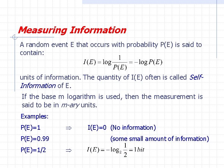
Measuring Information A random event E that occurs with probability P(E) is said to contain: units of information. The quantity of I(E) often is called Self. Information of E. If the base m logarithm is used, then the measurement is said to be in m-ary units. Examples: P(E)=1 P(E)=0. 99 P(E)=1/2 I(E)=0 (No information) (some small amount of information)

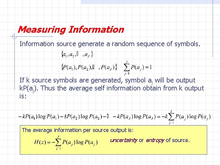
Measuring Information source generate a random sequence of symbols. If k source symbols are generated, symbol aj will be output k. P(aj). Thus the average self information obtain from k output is: The average information per source output is: uncertainty or entropy of source.

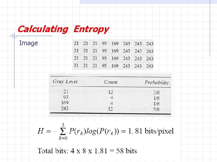
Calculating Entropy Image

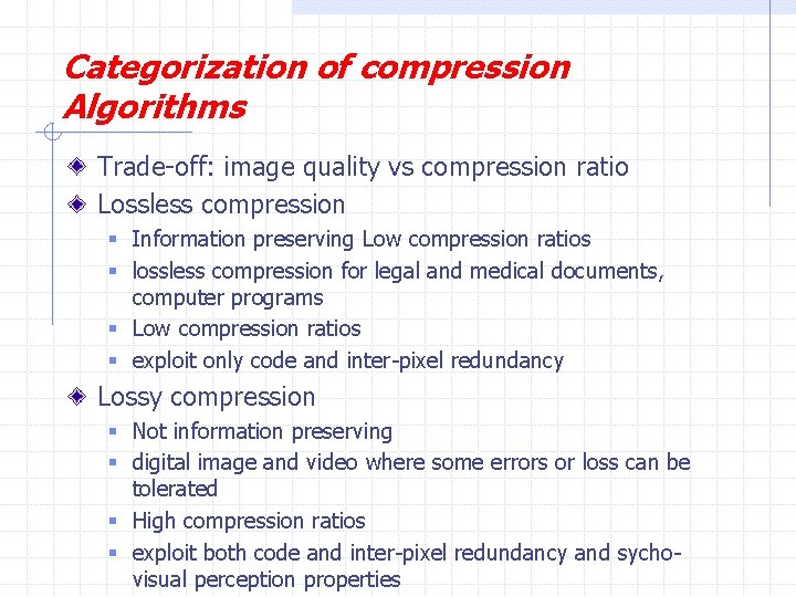
Categorization of compression Algorithms Trade-off: image quality vs compression ratio Lossless compression § Information preserving Low compression ratios § lossless compression for legal and medical documents, computer programs § Low compression ratios § exploit only code and inter-pixel redundancy Lossy compression § Not information preserving § digital image and video where some errors or loss can be tolerated § High compression ratios § exploit both code and inter-pixel redundancy and sychovisual perception properties

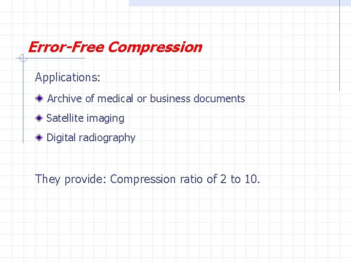
Error-Free Compression Applications: Archive of medical or business documents Satellite imaging Digital radiography They provide: Compression ratio of 2 to 10.

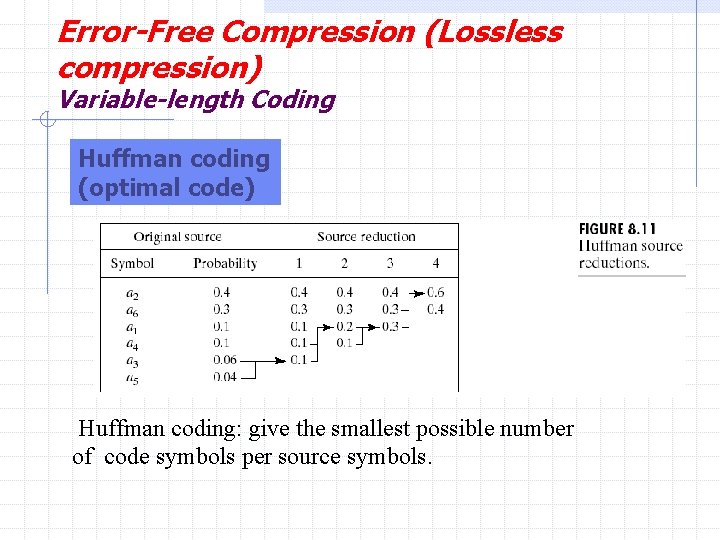
Error-Free Compression (Lossless compression) Variable-length Coding Huffman coding (optimal code) Huffman coding: give the smallest possible number of code symbols per source symbols.

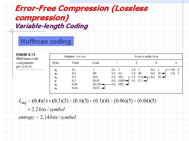
Error-Free Compression (Lossless compression) Variable-length Coding Huffman coding

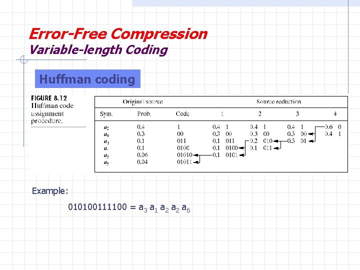
Error-Free Compression Variable-length Coding Huffman coding Example: 010100111100 = a 3 a 1 a 2 a 6

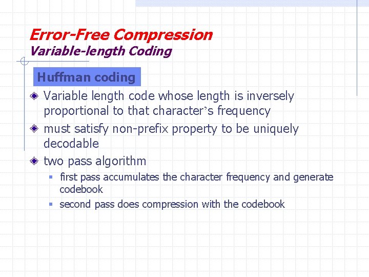
Error-Free Compression Variable-length Coding Huffman coding Variable length code whose length is inversely proportional to that character’s frequency must satisfy non-prefix property to be uniquely decodable two pass algorithm § first pass accumulates the character frequency and generate codebook § second pass does compression with the codebook

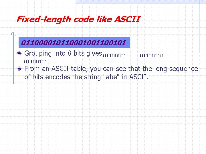
Fixed-length code like ASCII 01100001011000100101 Grouping into 8 bits gives 01100001 01100101 01100010 From an ASCII table, you can see that the long sequence of bits encodes the string "abe" in ASCII.

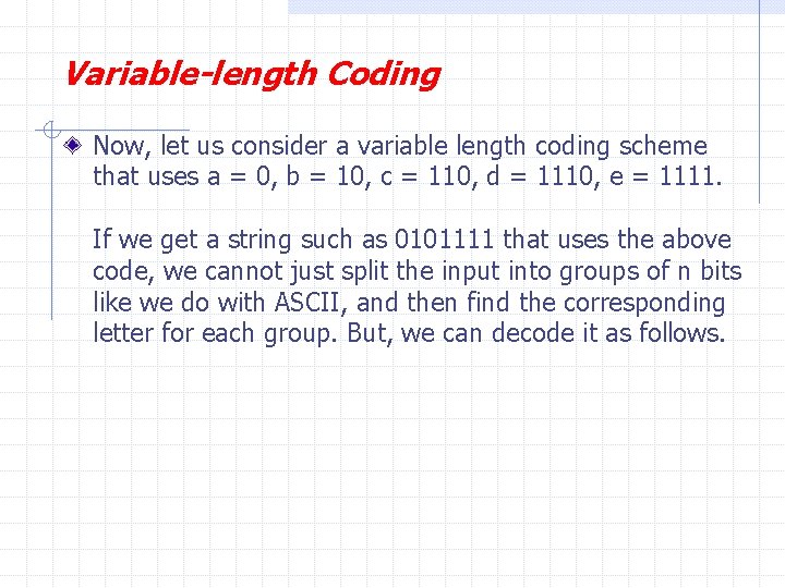
Variable-length Coding Now, let us consider a variable length coding scheme that uses a = 0, b = 10, c = 110, d = 1110, e = 1111. If we get a string such as 0101111 that uses the above code, we cannot just split the input into groups of n bits like we do with ASCII, and then find the corresponding letter for each group. But, we can decode it as follows.

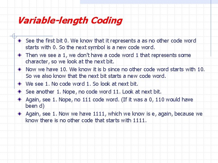
Variable-length Coding See the first bit 0. We know that it represents a as no other code word starts with 0. So the next symbol is a new code word. Then we see a 1, we don't have a code word 1 that represents some character, so we look at the next bit. Now we have 10. We know it is b since no other code word starts with 10. So we also know that the next bit starts a new code word. We see 1. No code word 1. So look at next bit. See another 1. Nope, no code word 11. Look at next bit. Again, see 1. Nope, no 111 code word. (If it was a 0, 110 would have been d) Again, see 1. Now we have 1111, which we know is e, again, because we know there is no other code that starts with 1111.

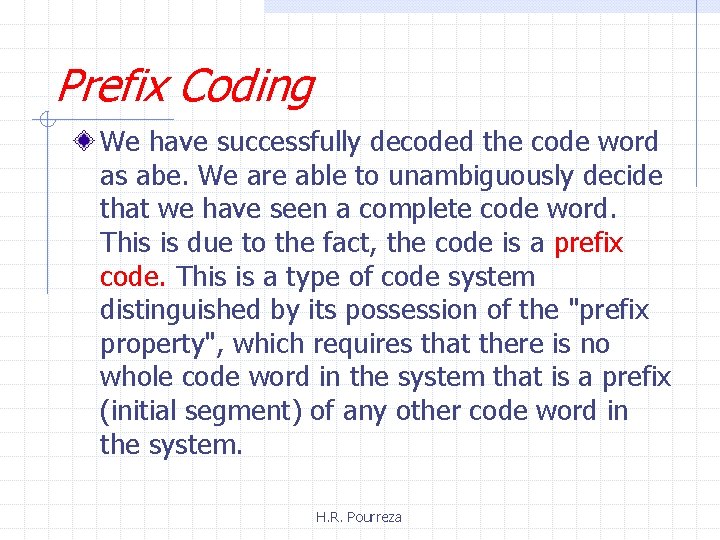
Prefix Coding We have successfully decoded the code word as abe. We are able to unambiguously decide that we have seen a complete code word. This is due to the fact, the code is a prefix code. This is a type of code system distinguished by its possession of the "prefix property", which requires that there is no whole code word in the system that is a prefix (initial segment) of any other code word in the system. H. R. Pourreza