Multiple Linear Regression Model The Multiple Regression Model

Multiple Linear Regression Model

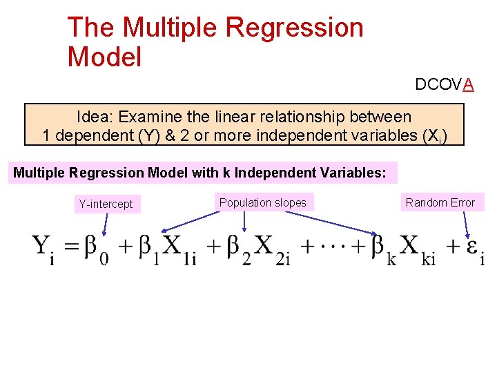
The Multiple Regression Model DCOVA Idea: Examine the linear relationship between 1 dependent (Y) & 2 or more independent variables (Xi) Multiple Regression Model with k Independent Variables: Y-intercept Population slopes Random Error

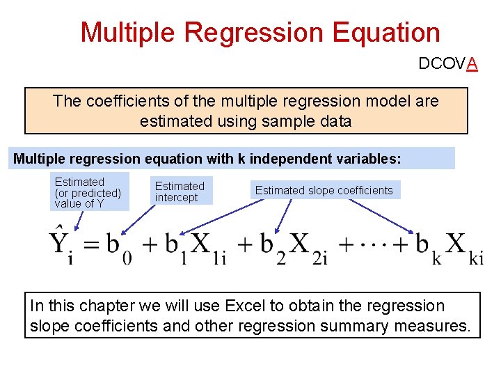
Multiple Regression Equation DCOVA The coefficients of the multiple regression model are estimated using sample data Multiple regression equation with k independent variables: Estimated (or predicted) value of Y Estimated intercept Estimated slope coefficients In this chapter we will use Excel to obtain the regression slope coefficients and other regression summary measures.

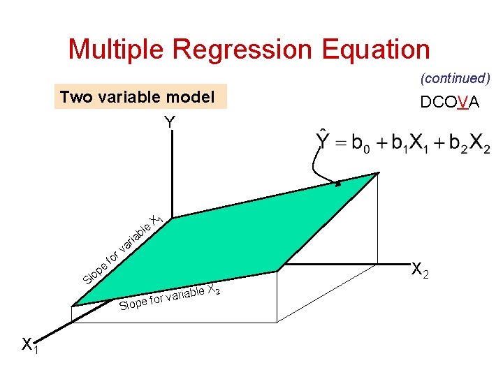
Multiple Regression Equation (continued) Two variable model DCOVA Y e p lo r fo ia ar le b v X 2 S le X 2 ariab e for v Slop X 1

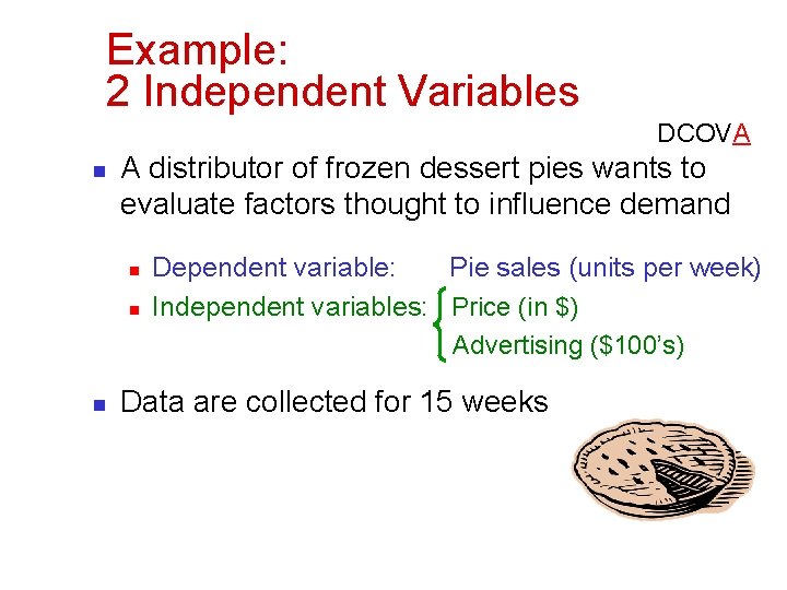
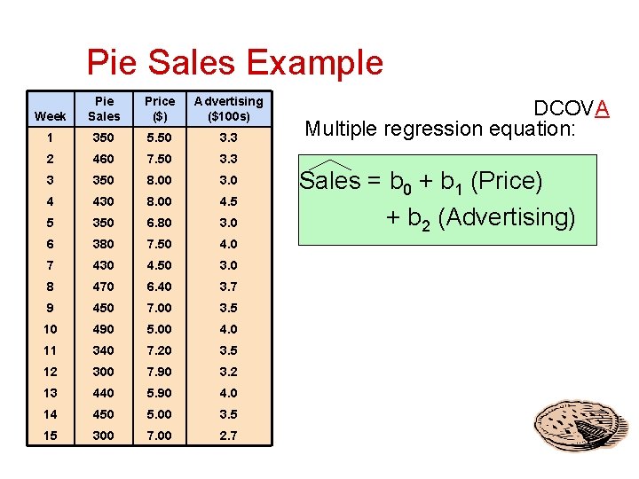
Example: 2 Independent Variables DCOVA n A distributor of frozen dessert pies wants to evaluate factors thought to influence demand n n n Dependent variable: Pie sales (units per week) Independent variables: Price (in $) Advertising ($100’s) Data are collected for 15 weeks

Pie Sales Example Week Pie Sales Price ($) Advertising ($100 s) 1 350 5. 50 3. 3 2 460 7. 50 3. 3 3 350 8. 00 3. 0 4 430 8. 00 4. 5 5 350 6. 80 3. 0 6 380 7. 50 4. 0 7 430 4. 50 3. 0 8 470 6. 40 3. 7 9 450 7. 00 3. 5 10 490 5. 00 4. 0 11 340 7. 20 3. 5 12 300 7. 90 3. 2 13 440 5. 90 4. 0 14 450 5. 00 3. 5 15 300 7. 00 2. 7 DCOVA Multiple regression equation: Sales = b 0 + b 1 (Price) + b 2 (Advertising)

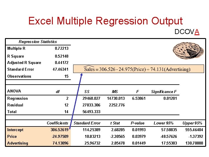
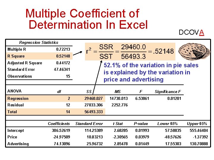
Excel Multiple Regression Output DCOVA Regression Statistics Multiple R 0. 72213 R Square 0. 52148 Adjusted R Square 0. 44172 Standard Error 47. 46341 Observations ANOVA Regression 15 df SS MS F 2 29460. 027 14730. 013 Residual 12 27033. 306 2252. 776 Total 14 56493. 333 Coefficients Standard Error Intercept 306. 52619 114. 25389 2. 68285 0. 01993 57. 58835 555. 46404 Price -24. 97509 10. 83213 -2. 30565 0. 03979 -48. 57626 -1. 37392 74. 13096 25. 96732 2. 85478 0. 01449 17. 55303 130. 70888 Advertising t Stat 6. 53861 Significance F P-value 0. 01201 Lower 95% Upper 95%

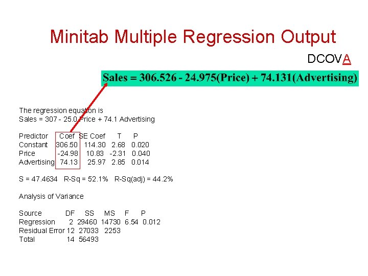
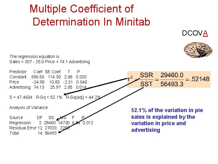
Minitab Multiple Regression Output DCOVA The regression equation is Sales = 307 - 25. 0 Price + 74. 1 Advertising Predictor Coef SE Coef T P Constant 306. 50 114. 30 2. 68 0. 020 Price -24. 98 10. 83 -2. 31 0. 040 Advertising 74. 13 25. 97 2. 85 0. 014 S = 47. 4634 R-Sq = 52. 1% R-Sq(adj) = 44. 2% Analysis of Variance Source DF SS MS F P Regression 2 29460 14730 6. 54 0. 012 Residual Error 12 27033 2253 Total 14 56493

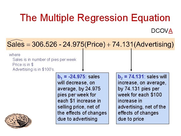
The Multiple Regression Equation DCOVA where Sales is in number of pies per week Price is in $ Advertising is in $100’s. b 1 = -24. 975: sales will decrease, on average, by 24. 975 pies per week for each $1 increase in selling price, net of the effects of changes due to advertising b 2 = 74. 131: sales will increase, on average, by 74. 131 pies per week for each $100 increase in advertising, net of the effects of changes due to price

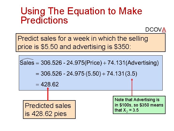
Using The Equation to Make Predictions DCOVA Predict sales for a week in which the selling price is $5. 50 and advertising is $350: Predicted sales is 428. 62 pies Note that Advertising is in $100 s, so $350 means that X 2 = 3. 5

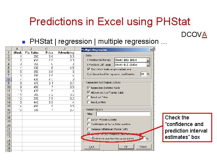
Predictions in Excel using PHStat n PHStat | regression | multiple regression … DCOVA Check the “confidence and prediction interval estimates” box

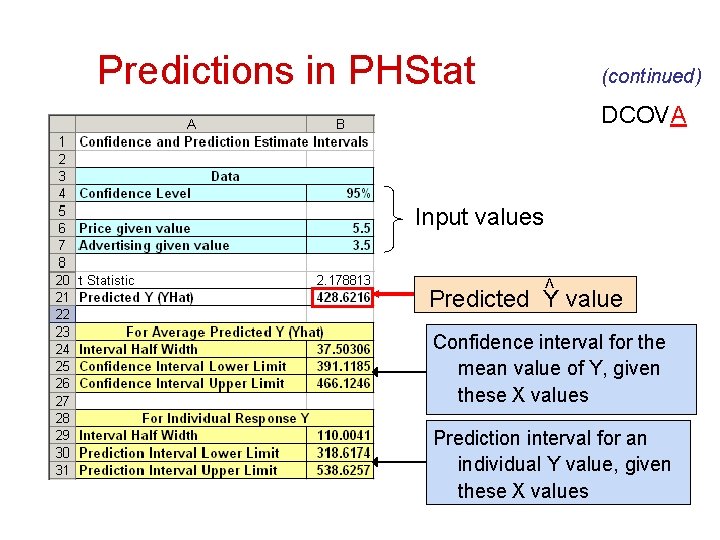
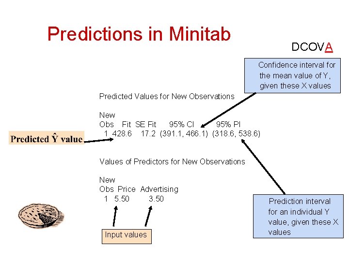
Predictions in PHStat (continued) DCOVA Input values < Predicted Y value Confidence interval for the mean value of Y, given these X values Prediction interval for an individual Y value, given these X values

Predictions in Minitab DCOVA Confidence interval for the mean value of Y, given these X values Predicted Values for New Observations New Obs Fit SE Fit 95% CI 95% PI 1 428. 6 17. 2 (391. 1, 466. 1) (318. 6, 538. 6) Values of Predictors for New Observations New Obs Price Advertising 1 5. 50 3. 50 Input values Prediction interval for an individual Y value, given these X values

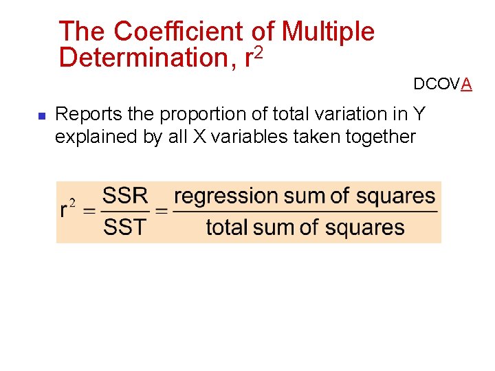
The Coefficient of Multiple Determination, r 2 DCOVA n Reports the proportion of total variation in Y explained by all X variables taken together

Multiple Coefficient of Determination In Excel DCOVA Regression Statistics Multiple R 0. 72213 R Square 0. 52148 Adjusted R Square 0. 44172 Standard Error Observations ANOVA Regression 52. 1% of the variation in pie sales is explained by the variation in price and advertising 47. 46341 15 df SS MS F 2 29460. 027 14730. 013 Residual 12 27033. 306 2252. 776 Total 14 56493. 333 Coefficients Standard Error Intercept 306. 52619 114. 25389 2. 68285 0. 01993 57. 58835 555. 46404 Price -24. 97509 10. 83213 -2. 30565 0. 03979 -48. 57626 -1. 37392 74. 13096 25. 96732 2. 85478 0. 01449 17. 55303 130. 70888 Advertising t Stat 6. 53861 Significance F P-value 0. 01201 Lower 95% Upper 95%

Multiple Coefficient of Determination In Minitab DCOVA The regression equation is Sales = 307 - 25. 0 Price + 74. 1 Advertising Predictor Coef SE Coef T P Constant 306. 50 114. 30 2. 68 0. 020 Price -24. 98 10. 83 -2. 31 0. 040 Advertising 74. 13 25. 97 2. 85 0. 014 S = 47. 4634 R-Sq = 52. 1% R-Sq(adj) = 44. 2% Analysis of Variance Source DF SS MS F P Regression 2 29460 14730 6. 54 0. 012 Residual Error 12 27033 2253 Total 14 56493 52. 1% of the variation in pie sales is explained by the variation in price and advertising

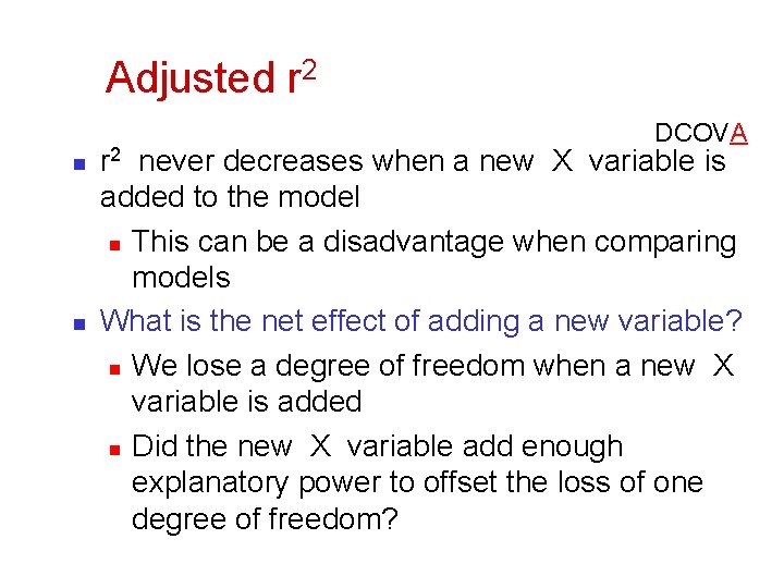
Adjusted r 2 DCOVA n n r 2 never decreases when a new X variable is added to the model n This can be a disadvantage when comparing models What is the net effect of adding a new variable? n We lose a degree of freedom when a new X variable is added n Did the new X variable add enough explanatory power to offset the loss of one degree of freedom?

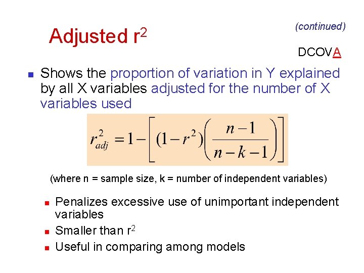
Adjusted r 2 n (continued) DCOVA Shows the proportion of variation in Y explained by all X variables adjusted for the number of X variables used (where n = sample size, k = number of independent variables) n n n Penalizes excessive use of unimportant independent variables Smaller than r 2 Useful in comparing among models

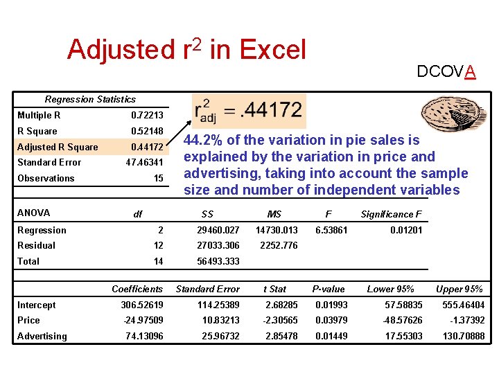
Adjusted r 2 in Excel DCOVA Regression Statistics Multiple R 0. 72213 R Square 0. 52148 Adjusted R Square 0. 44172 Standard Error 47. 46341 Observations ANOVA Regression 15 df 44. 2% of the variation in pie sales is explained by the variation in price and advertising, taking into account the sample size and number of independent variables SS MS F 2 29460. 027 14730. 013 Residual 12 27033. 306 2252. 776 Total 14 56493. 333 Coefficients Standard Error Intercept 306. 52619 114. 25389 2. 68285 0. 01993 57. 58835 555. 46404 Price -24. 97509 10. 83213 -2. 30565 0. 03979 -48. 57626 -1. 37392 74. 13096 25. 96732 2. 85478 0. 01449 17. 55303 130. 70888 Advertising t Stat 6. 53861 Significance F P-value 0. 01201 Lower 95% Upper 95%

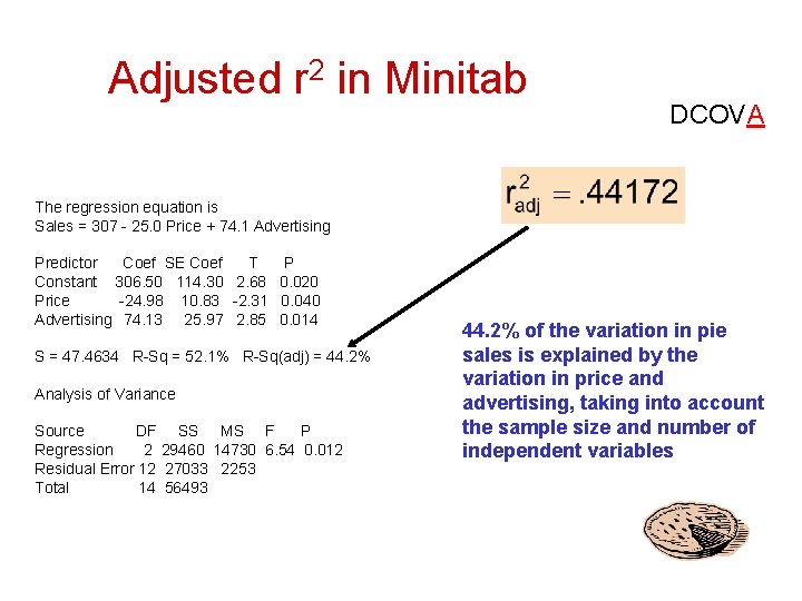
Adjusted r 2 in Minitab DCOVA The regression equation is Sales = 307 - 25. 0 Price + 74. 1 Advertising Predictor Coef SE Coef T P Constant 306. 50 114. 30 2. 68 0. 020 Price -24. 98 10. 83 -2. 31 0. 040 Advertising 74. 13 25. 97 2. 85 0. 014 S = 47. 4634 R-Sq = 52. 1% R-Sq(adj) = 44. 2% Analysis of Variance Source DF SS MS F P Regression 2 29460 14730 6. 54 0. 012 Residual Error 12 27033 2253 Total 14 56493 44. 2% of the variation in pie sales is explained by the variation in price and advertising, taking into account the sample size and number of independent variables

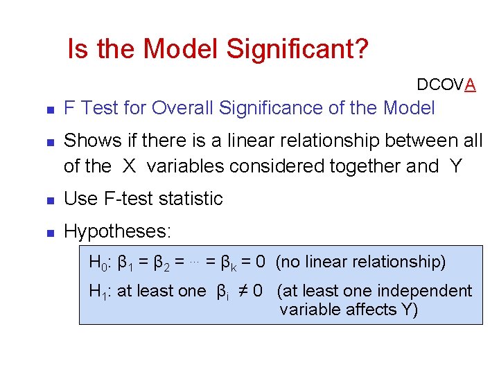
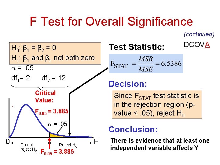
Is the Model Significant? DCOVA n n F Test for Overall Significance of the Model Shows if there is a linear relationship between all of the X variables considered together and Y n Use F-test statistic n Hypotheses: H 0: β 1 = β 2 = … = βk = 0 (no linear relationship) H 1: at least one βi ≠ 0 (at least one independent variable affects Y)

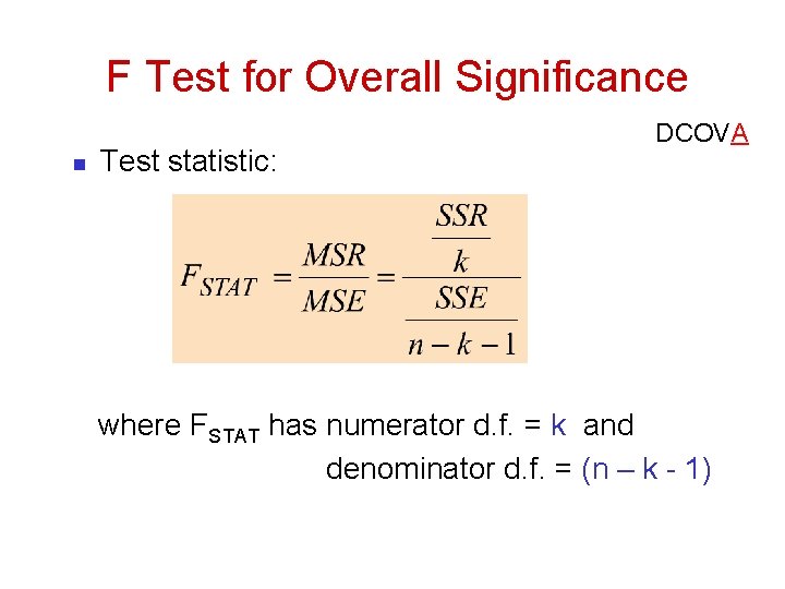
F Test for Overall Significance n Test statistic: DCOVA where FSTAT has numerator d. f. = k and denominator d. f. = (n – k - 1)

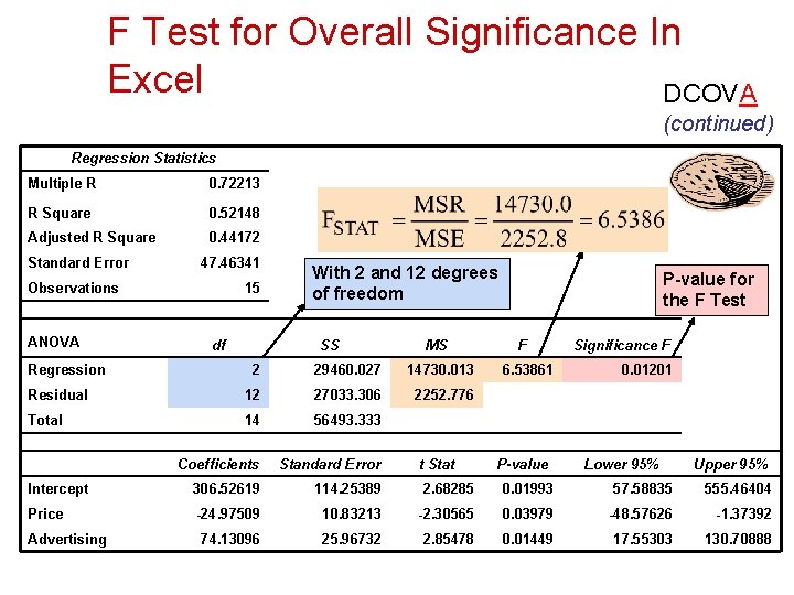
F Test for Overall Significance In Excel DCOVA (continued) Regression Statistics Multiple R 0. 72213 R Square 0. 52148 Adjusted R Square 0. 44172 Standard Error 47. 46341 Observations ANOVA Regression 15 df With 2 and 12 degrees of freedom SS MS P-value for the F Test F 2 29460. 027 14730. 013 Residual 12 27033. 306 2252. 776 Total 14 56493. 333 Coefficients Standard Error Intercept 306. 52619 114. 25389 2. 68285 0. 01993 57. 58835 555. 46404 Price -24. 97509 10. 83213 -2. 30565 0. 03979 -48. 57626 -1. 37392 74. 13096 25. 96732 2. 85478 0. 01449 17. 55303 130. 70888 Advertising t Stat 6. 53861 Significance F P-value 0. 01201 Lower 95% Upper 95%

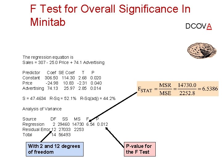
F Test for Overall Significance In Minitab DCOVA The regression equation is Sales = 307 - 25. 0 Price + 74. 1 Advertising Predictor Coef SE Coef T P Constant 306. 50 114. 30 2. 68 0. 020 Price -24. 98 10. 83 -2. 31 0. 040 Advertising 74. 13 25. 97 2. 85 0. 014 S = 47. 4634 R-Sq = 52. 1% R-Sq(adj) = 44. 2% Analysis of Variance Source DF SS MS F P Regression 2 29460 14730 6. 54 0. 012 Residual Error 12 27033 2253 Total 14 56493 With 2 and 12 degrees of freedom P-value for the F Test

F Test for Overall Significance (continued) H 0: β 1 = β 2 = 0 H 1: β 1 and β 2 not both zero =. 05 df 1= 2 df 2 = 12 Critical Value: =. 05 Do not reject H 0 Reject H 0 F 0. 05 = 3. 885 DCOVA Decision: Since FSTAT test statistic is in the rejection region (pvalue <. 05), reject H 0 F 0. 05 = 3. 885 0 Test Statistic: Conclusion: F There is evidence that at least one independent variable affects Y

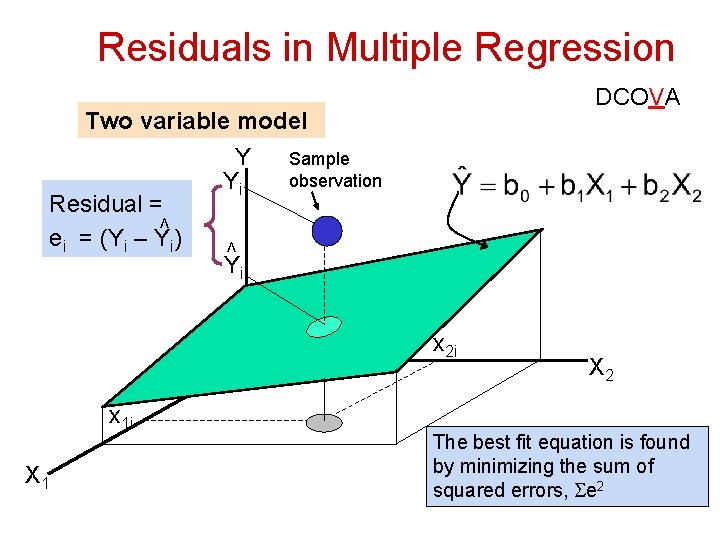
Residuals in Multiple Regression DCOVA Two variable model Sample observation < Residual = ei = (Yi – Yi) Y Yi < Yi x 2 i x 1 i X 1 X 2 The best fit equation is found by minimizing the sum of squared errors, e 2

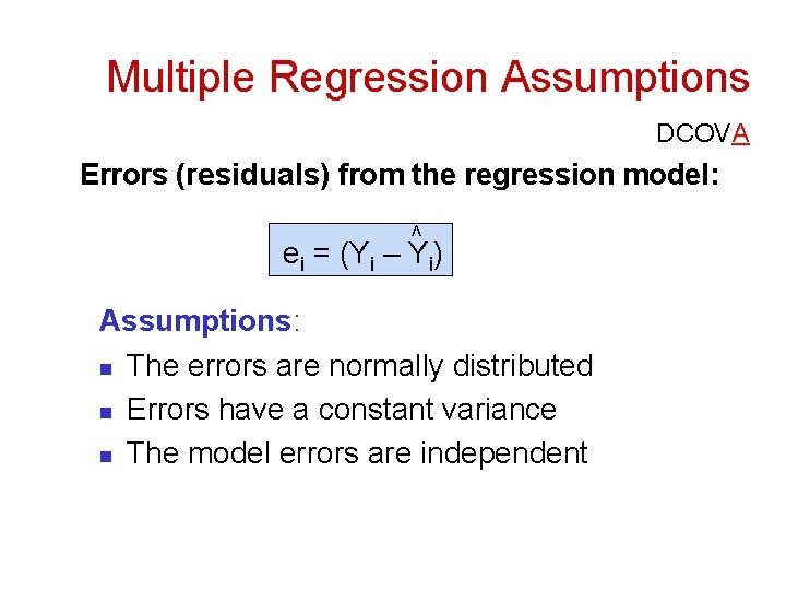
Multiple Regression Assumptions DCOVA Errors (residuals) from the regression model: < ei = (Yi – Yi) Assumptions: n The errors are normally distributed n Errors have a constant variance n The model errors are independent

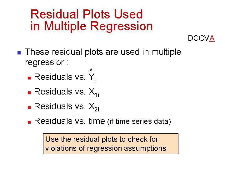
Residual Plots Used in Multiple Regression DCOVA n These residual plots are used in multiple regression: < n Residuals vs. Yi n Residuals vs. X 1 i n Residuals vs. X 2 i n Residuals vs. time (if time series data) Use the residual plots to check for violations of regression assumptions

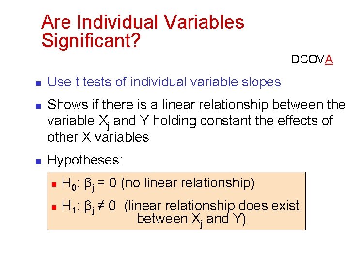
Are Individual Variables Significant? DCOVA n n n Use t tests of individual variable slopes Shows if there is a linear relationship between the variable Xj and Y holding constant the effects of other X variables Hypotheses: n n H 0: βj = 0 (no linear relationship) H 1: βj ≠ 0 (linear relationship does exist between Xj and Y)

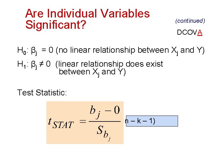
Are Individual Variables Significant? (continued) DCOVA H 0: βj = 0 (no linear relationship between Xj and Y) H 1: βj ≠ 0 (linear relationship does exist between Xj and Y) Test Statistic: (df = n – k – 1)

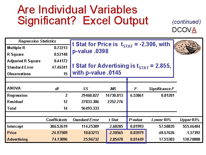
Are Individual Variables Significant? Excel Output Regression Statistics Multiple R 0. 72213 R Square 0. 52148 Adjusted R Square 0. 44172 Standard Error 47. 46341 Observations ANOVA Regression 15 df (continued) DCOVA t Stat for Price is t. STAT = -2. 306, with p-value. 0398 t Stat for Advertising is t. STAT = 2. 855, with p-value. 0145 SS MS F 2 29460. 027 14730. 013 Residual 12 27033. 306 2252. 776 Total 14 56493. 333 Coefficients Standard Error Intercept 306. 52619 114. 25389 2. 68285 0. 01993 57. 58835 555. 46404 Price -24. 97509 10. 83213 -2. 30565 0. 03979 -48. 57626 -1. 37392 74. 13096 25. 96732 2. 85478 0. 01449 17. 55303 130. 70888 Advertising t Stat 6. 53861 Significance F P-value 0. 01201 Lower 95% Upper 95%

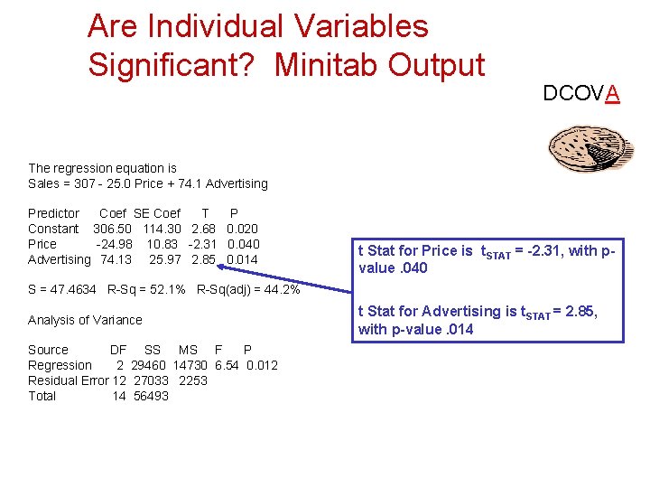
Are Individual Variables Significant? Minitab Output DCOVA The regression equation is Sales = 307 - 25. 0 Price + 74. 1 Advertising Predictor Coef SE Coef T P Constant 306. 50 114. 30 2. 68 0. 020 Price -24. 98 10. 83 -2. 31 0. 040 Advertising 74. 13 25. 97 2. 85 0. 014 t Stat for Price is t. STAT = -2. 31, with pvalue. 040 S = 47. 4634 R-Sq = 52. 1% R-Sq(adj) = 44. 2% Analysis of Variance Source DF SS MS F P Regression 2 29460 14730 6. 54 0. 012 Residual Error 12 27033 2253 Total 14 56493 t Stat for Advertising is t. STAT = 2. 85, with p-value. 014

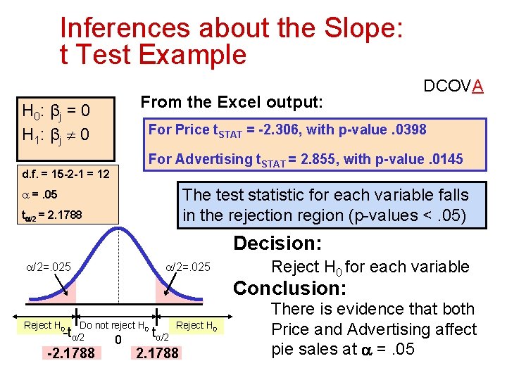
Inferences about the Slope: t Test Example From the Excel output: H 0: β j = 0 H 1: β j 0 DCOVA For Price t. STAT = -2. 306, with p-value. 0398 For Advertising t. STAT = 2. 855, with p-value. 0145 d. f. = 15 -2 -1 = 12 The test statistic for each variable falls in the rejection region (p-values <. 05) =. 05 t /2 = 2. 1788 Decision: /2=. 025 Reject H 0 for each variable Conclusion: Reject H 0 Do not reject H 0 -tα/2 -2. 1788 0 Reject H 0 tα/2 2. 1788 There is evidence that both Price and Advertising affect pie sales at =. 05

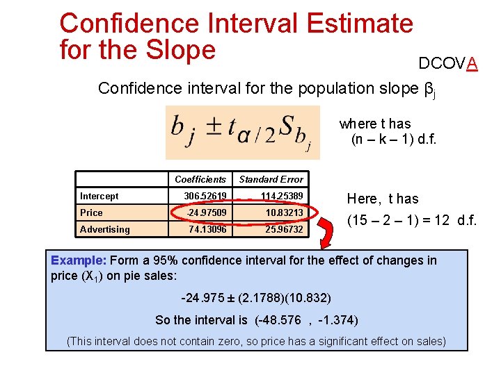
Confidence Interval Estimate for the Slope DCOVA Confidence interval for the population slope βj where t has (n – k – 1) d. f. Coefficients Standard Error Intercept 306. 52619 114. 25389 Price -24. 97509 10. 83213 74. 13096 25. 96732 Advertising Here, t has (15 – 2 – 1) = 12 d. f. Example: Form a 95% confidence interval for the effect of changes in price (X 1) on pie sales: -24. 975 ± (2. 1788)(10. 832) So the interval is (-48. 576 , -1. 374) (This interval does not contain zero, so price has a significant effect on sales)

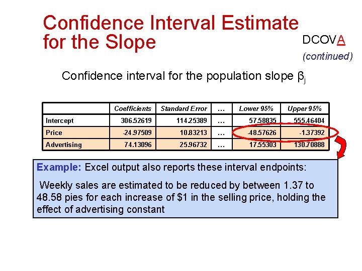
Confidence Interval Estimate DCOVA for the Slope (continued) Confidence interval for the population slope βj Coefficients Standard Error … Intercept 306. 52619 114. 25389 … 57. 58835 555. 46404 Price -24. 97509 10. 83213 … -48. 57626 -1. 37392 74. 13096 25. 96732 … 17. 55303 130. 70888 Advertising Lower 95% Upper 95% Example: Excel output also reports these interval endpoints: Weekly sales are estimated to be reduced by between 1. 37 to 48. 58 pies for each increase of $1 in the selling price, holding the effect of advertising constant

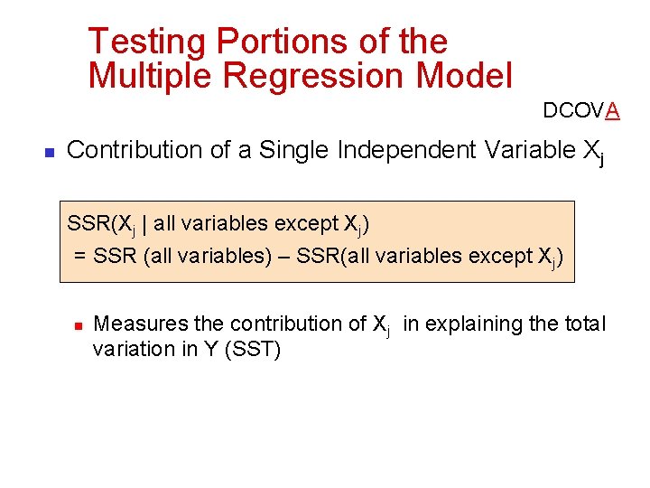
Testing Portions of the Multiple Regression Model DCOVA n Contribution of a Single Independent Variable Xj SSR(Xj | all variables except Xj) = SSR (all variables) – SSR(all variables except Xj) n Measures the contribution of Xj in explaining the total variation in Y (SST)

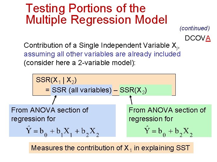
Testing Portions of the Multiple Regression Model (continued) Contribution of a Single Independent Variable Xj, assuming all other variables are already included (consider here a 2 -variable model): DCOVA SSR(X 1 | X 2) = SSR (all variables) – SSR(X 2) From ANOVA section of regression for Measures the contribution of X 1 in explaining SST

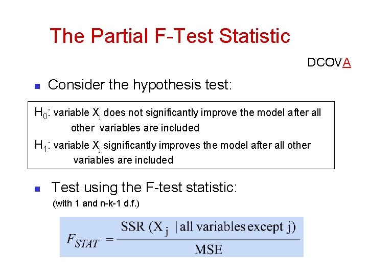
The Partial F-Test Statistic DCOVA n Consider the hypothesis test: H 0: variable Xj does not significantly improve the model after all other variables are included H 1: variable Xj significantly improves the model after all other variables are included n Test using the F-test statistic: (with 1 and n-k-1 d. f. )

Testing Portions of Model: Example DCOVA Example: Frozen dessert pies Test at the =. 05 level to determine whether the price variable significantly improves the model given that advertising is included

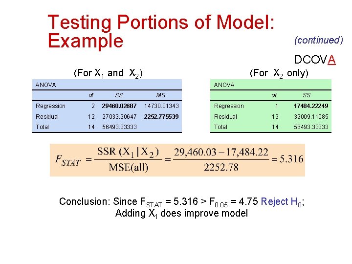
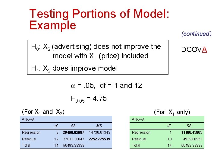
Testing Portions of Model: Example (continued) H 0: X 1 (price) does not improve the model with X 2 (advertising) included DCOVA H 1: X 1 does improve model =. 05, df = 1 and 12 F 0. 05 = 4. 75 (For X 1 and X 2) (For X 2 only) ANOVA df SS MS 2 29460. 02687 14730. 01343 Regression Residual 12 27033. 30647 2252. 775539 Total 14 56493. 33333 Regression df SS 1 17484. 22249 Residual 13 39009. 11085 Total 14 56493. 33333

Testing Portions of Model: Example (continued) DCOVA (For X 1 and X 2) (For X 2 only) ANOVA df SS MS 2 29460. 02687 14730. 01343 Regression Residual 12 27033. 30647 2252. 775539 Total 14 56493. 33333 Regression df SS 1 17484. 22249 Residual 13 39009. 11085 Total 14 56493. 33333 Conclusion: Since FSTAT = 5. 316 > F 0. 05 = 4. 75 Reject H 0; Adding X 1 does improve model

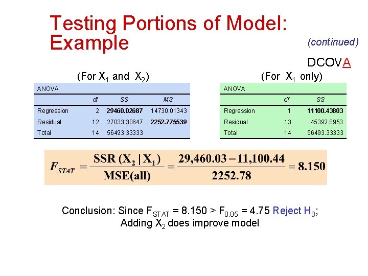
Testing Portions of Model: Example (continued) H 0: X 2 (advertising) does not improve the model with X 1 (price) included DCOVA H 1: X 2 does improve model =. 05, df = 1 and 12 F 0. 05 = 4. 75 (For X 1 and X 2) (For X 1 only) ANOVA df SS MS 2 29460. 02687 14730. 01343 Regression Residual 12 27033. 30647 2252. 775539 Total 14 56493. 33333 Regression df SS 1 11100. 43803 Residual 13 45392. 8953 Total 14 56493. 33333

Testing Portions of Model: Example (continued) DCOVA (For X 1 and X 2) (For X 1 only) ANOVA df SS MS 2 29460. 02687 14730. 01343 Regression Residual 12 27033. 30647 2252. 775539 Total 14 56493. 33333 Regression df SS 1 11100. 43803 Residual 13 45392. 8953 Total 14 56493. 33333 Conclusion: Since FSTAT = 8. 150 > F 0. 05 = 4. 75 Reject H 0; Adding X 2 does improve model

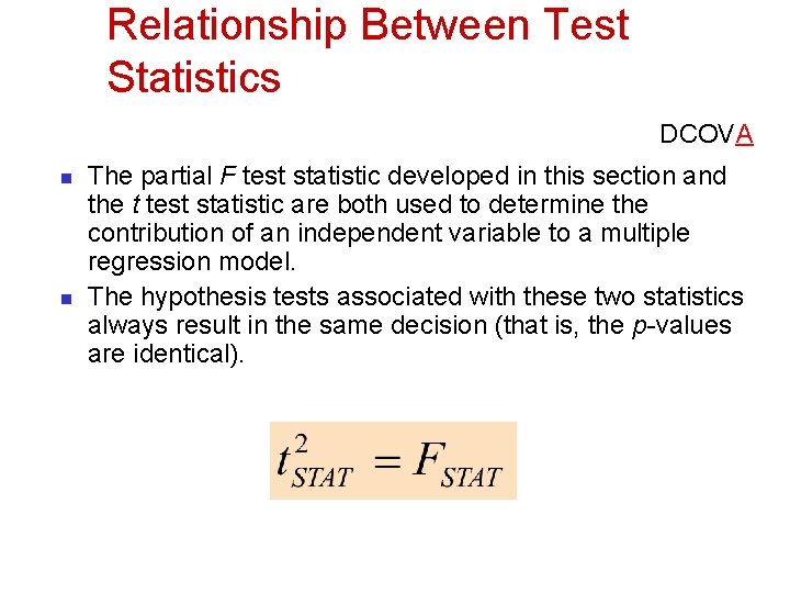
Relationship Between Test Statistics DCOVA n n The partial F test statistic developed in this section and the t test statistic are both used to determine the contribution of an independent variable to a multiple regression model. The hypothesis tests associated with these two statistics always result in the same decision (that is, the p-values are identical).

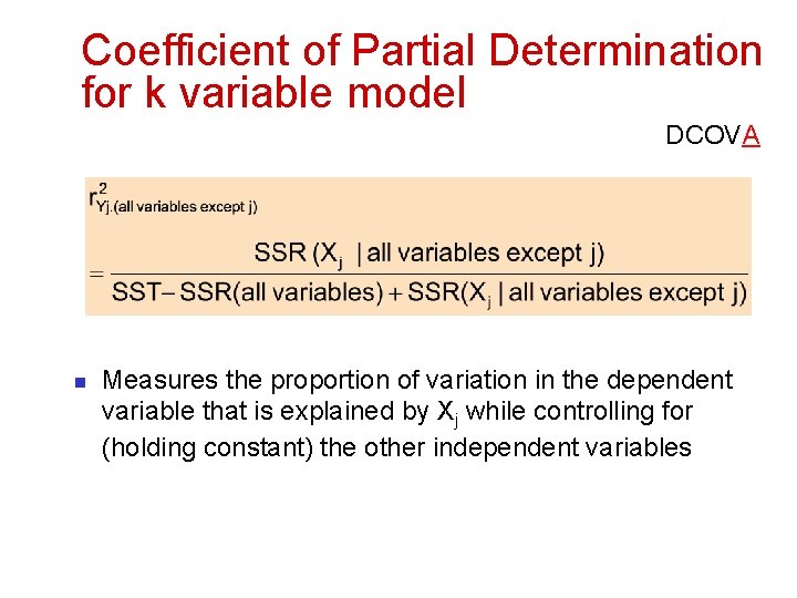
Coefficient of Partial Determination for k variable model DCOVA n Measures the proportion of variation in the dependent variable that is explained by Xj while controlling for (holding constant) the other independent variables

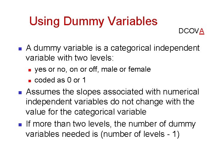
Using Dummy Variables n A dummy variable is a categorical independent variable with two levels: n n DCOVA yes or no, on or off, male or female coded as 0 or 1 Assumes the slopes associated with numerical independent variables do not change with the value for the categorical variable If more than two levels, the number of dummy variables needed is (number of levels - 1)

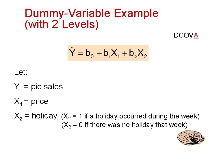
Dummy-Variable Example (with 2 Levels) DCOVA Let: Y = pie sales X 1 = price X 2 = holiday (X 2 = 1 if a holiday occurred during the week) (X 2 = 0 if there was no holiday that week)

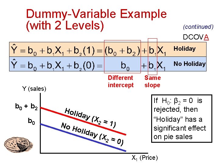
Dummy-Variable Example (with 2 Levels) (continued) DCOVA Holiday No Holiday Different intercept Y (sales) b 0 + b 2 b 0 Holi da y (X 2 No H o liday = 1) (X = 2 0) Same slope If H 0: β 2 = 0 is rejected, then “Holiday” has a significant effect on pie sales X 1 (Price)

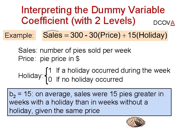
Interpreting the Dummy Variable Coefficient (with 2 Levels) DCOVA Example: Sales: number of pies sold per week Price: pie price in $ 1 If a holiday occurred during the week Holiday: 0 If no holiday occurred b 2 = 15: on average, sales were 15 pies greater in weeks with a holiday than in weeks without a holiday, given the same price

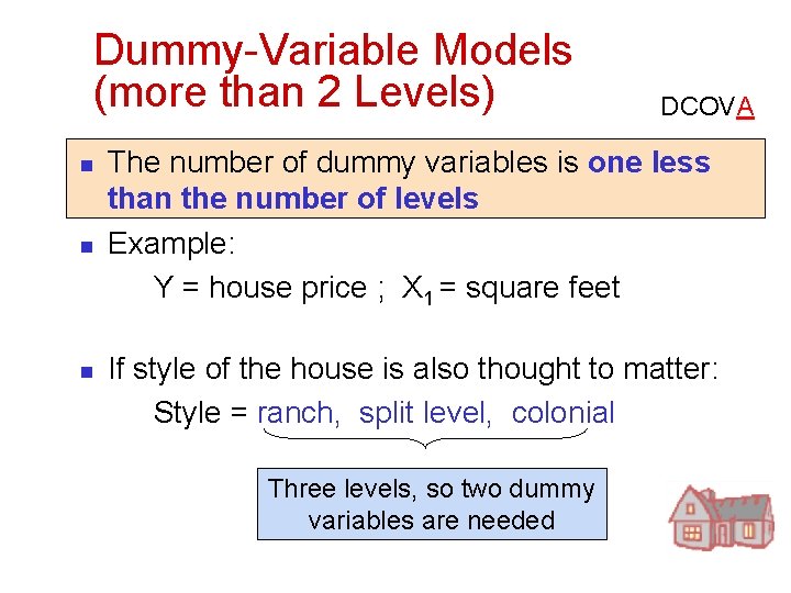
Dummy-Variable Models (more than 2 Levels) n n n DCOVA The number of dummy variables is one less than the number of levels Example: Y = house price ; X 1 = square feet If style of the house is also thought to matter: Style = ranch, split level, colonial Three levels, so two dummy variables are needed

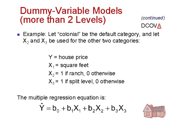
Dummy-Variable Models (more than 2 Levels) n (continued) DCOVA Example: Let “colonial” be the default category, and let X 2 and X 3 be used for the other two categories: Y = house price X 1 = square feet X 2 = 1 if ranch, 0 otherwise X 3 = 1 if split level, 0 otherwise The multiple regression equation is:

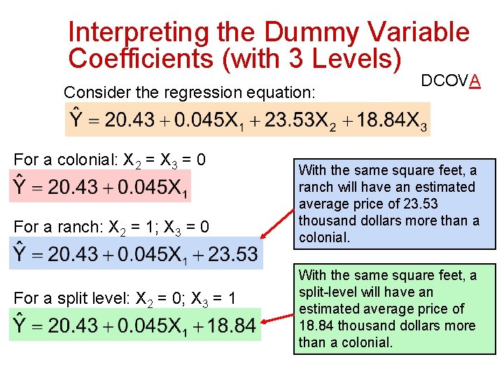
Interpreting the Dummy Variable Coefficients (with 3 Levels) Consider the regression equation: For a colonial: X 2 = X 3 = 0 For a ranch: X 2 = 1; X 3 = 0 For a split level: X 2 = 0; X 3 = 1 DCOVA With the same square feet, a ranch will have an estimated average price of 23. 53 thousand dollars more than a colonial. With the same square feet, a split-level will have an estimated average price of 18. 84 thousand dollars more than a colonial.

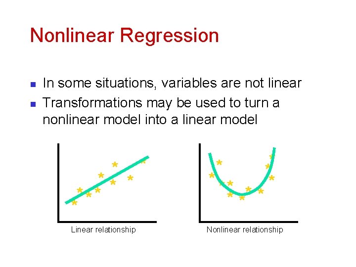
Nonlinear Regression n n In some situations, variables are not linear Transformations may be used to turn a nonlinear model into a linear model * *** * Linear relationship * ** * * * * Nonlinear relationship

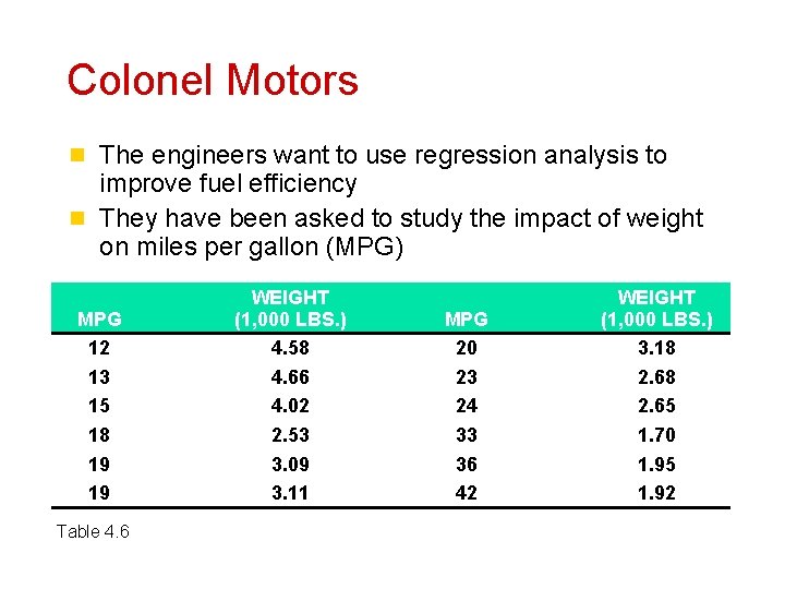
Colonel Motors n The engineers want to use regression analysis to improve fuel efficiency n They have been asked to study the impact of weight on miles per gallon (MPG) MPG 12 13 15 18 19 19 Table 4. 6 WEIGHT (1, 000 LBS. ) 4. 58 4. 66 4. 02 2. 53 3. 09 3. 11 MPG 20 23 24 33 36 42 WEIGHT (1, 000 LBS. ) 3. 18 2. 65 1. 70 1. 95 1. 92

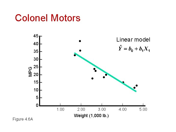
Colonel Motors 45 – 40 – 35 – 30 – MPG Linear model 25 – 20 – 15 – 10 – 5– 0– Figure 4. 6 A | | | 1. 00 2. 00 3. 00 4. 00 5. 00 Weight (1, 000 lb. )

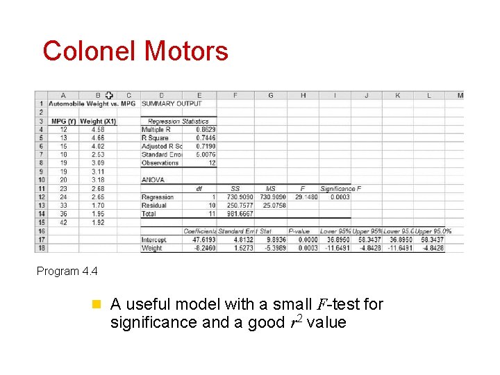
Colonel Motors Program 4. 4 n A useful model with a small F-test for significance and a good r 2 value

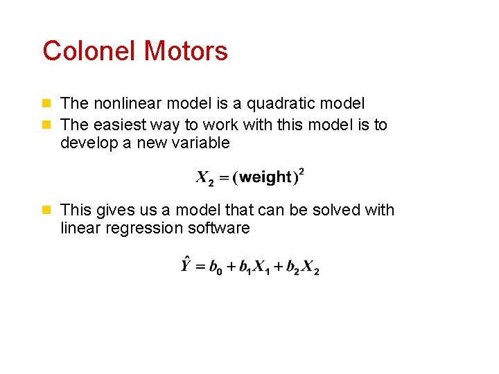
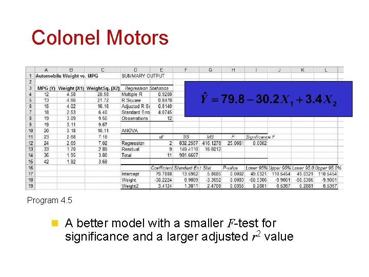
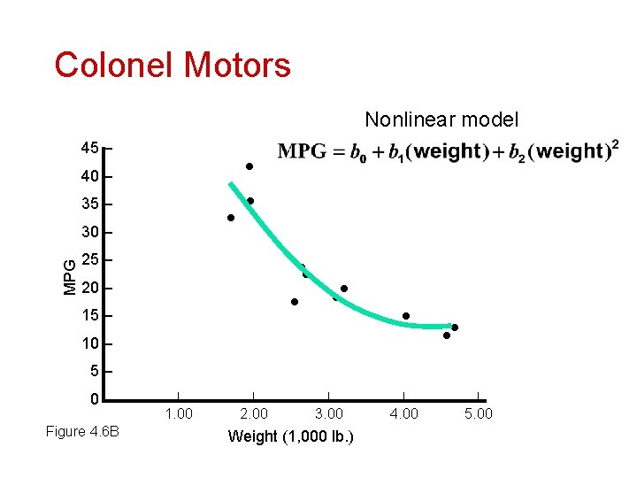
Colonel Motors n The nonlinear model is a quadratic model n The easiest way to work with this model is to develop a new variable n This gives us a model that can be solved with linear regression software

Colonel Motors Program 4. 5 n A better model with a smaller F-test for significance and a larger adjusted r 2 value

Colonel Motors Nonlinear model 45 – 40 – 35 – MPG 30 – 25 – 20 – 15 – 10 – 5– 0– Figure 4. 6 B | | | 1. 00 2. 00 3. 00 4. 00 5. 00 Weight (1, 000 lb. )

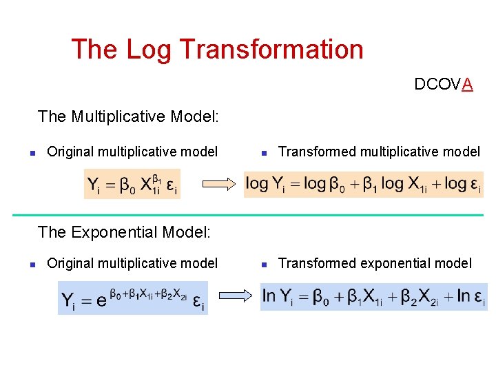
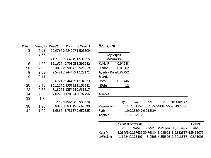
The Log Transformation DCOVA The Multiplicative Model: n Original multiplicative model n Transformed exponential model The Exponential Model: n Original multiplicative model

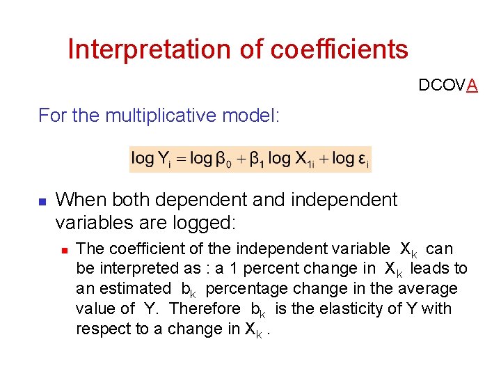
Interpretation of coefficients DCOVA For the multiplicative model: n When both dependent and independent variables are logged: n The coefficient of the independent variable Xk can be interpreted as : a 1 percent change in Xk leads to an estimated bk percentage change in the average value of Y. Therefore bk is the elasticity of Y with respect to a change in Xk.

MPG 12 13 15 18 19 19 20 23 24 33 36 42 Weights Weig 2 ln. MPG Ln. Weight 20. 9764 2. 484907 1. 521699 4. 58 4. 66 21. 7156 2. 564949 1. 539015 16. 1604 2. 70805 1. 391282 4. 02 6. 4009 2. 890372 0. 928219 2. 53 9. 5481 2. 944439 1. 128171 3. 09 3. 11 9. 6721 2. 944439 1. 134623 10. 1124 2. 995732 1. 156881 3. 18 7. 1824 3. 135494 0. 985817 2. 68 7. 0225 3. 178054 0. 97456 2. 65 1. 7 2. 89 3. 496508 0. 530628 3. 8025 3. 583519 0. 667829 1. 95 3. 6864 3. 73767 0. 652325 1. 92 ÖZET ÇIKIŞI Regresyon İstatistikleri Çoklu R 0. 94288 R Kare 0. 88902 Ayarlı R Kare 0. 87792 Standart Hata 0. 13746 Gözlem 12 ANOVA df Regresyon Fark Toplam Kesişim Ln. Weight SS MS F Anlamlılık F 1 1. 51357 80. 10787 4. 3492 E-06 10 0. 188942 0. 018894 11 1. 702512 Katsayıl Standart Yüksek ar Hata t Stat P-değeri Düşük %95 4. 23493 0. 137637 30. 76884 3. 08 E-11 3. 9282587 4. 5416077 -1. 1224 0. 125407 -8. 9503 4. 35 E-06 -1. 4018587 -0. 843008