Multivariate Regression Multivariate Regression We have learned how

Multivariate Regression

Multivariate Regression • We have learned how to use OLS for two variables, known as bivariate regression. • We have seen that OLS regression is a powerful and flexible tool for summarizing relationships between a dependent and independent variable. As a technique for measuring covariation, it can help us to establish causality between two variables.

Multivariate Regression • Using only two variables can be problematic, however, for two reasons: • There may be multiple causes of the dependent variable. In our income examples, we used education and experience separately as independent or explanatory variables. • If we exclude a relevant variable from our regression equation, however, our estimate of the impact X on Y will be biased. Consequently, we may over(under)state the impact the independent variable has on the dependent variable if we exclude a relevant variable.

Regression and Causality • Recall establishing causality requires ruling out nonspuriousness. • In a bivariate model, however, it is difficult to rule out nonspuriousness. • Multivariate regression is a powerful tool for reducing the likelihood that a causal relationship that we observe is really a spurious one.

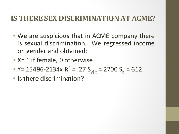
IS THERE SEX DISCRIMINATION AT ACME? • We are suspicious that in ACME company there is sexual discrimination. We regressed income on gender and obtained: • X= 1 if female, 0 otherwise • Y= 15496 -2134 x R 2 =. 27 Sy|x = 2700 Sb = 612 • Is there discrimination?

SEX DISCRIMINATION AT ACME • Clearly, women earn less than men. • Coefficient for gender is statistically significant. • Coefficient for gender is substantively meaningful • Should we proceed with a lawsuit? How might the defense lawyers for ACME try to defend their client?

Defending Acme • Acme could argue that gender differences in earnings are due to gender differences in: • Experience • Education • Skill, etc. • The apparent relationship between gender and income is spurious • Acme hires a lawyer who argues that women have less experience

MULTIVARIATE REGRESSION • In multivariate regression the objective is still to estimate the line that minimizes the amount of errors in our predictions. We again employ the least squares principle. In multivariate regression, however, we are working with more than two dimensions. The regression line is now expressed as:

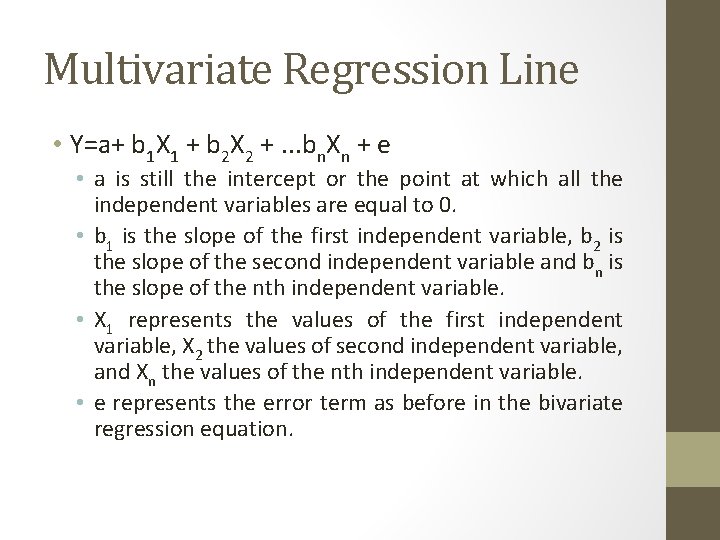
Multivariate Regression Line • Y=a+ b 1 X 1 + b 2 X 2 +. . . bn. Xn + e • a is still the intercept or the point at which all the independent variables are equal to 0. • b 1 is the slope of the first independent variable, b 2 is the slope of the second independent variable and bn is the slope of the nth independent variable. • X 1 represents the values of the first independent variable, X 2 the values of second independent variable, and Xn the values of the nth independent variable. • e represents the error term as before in the bivariate regression equation.

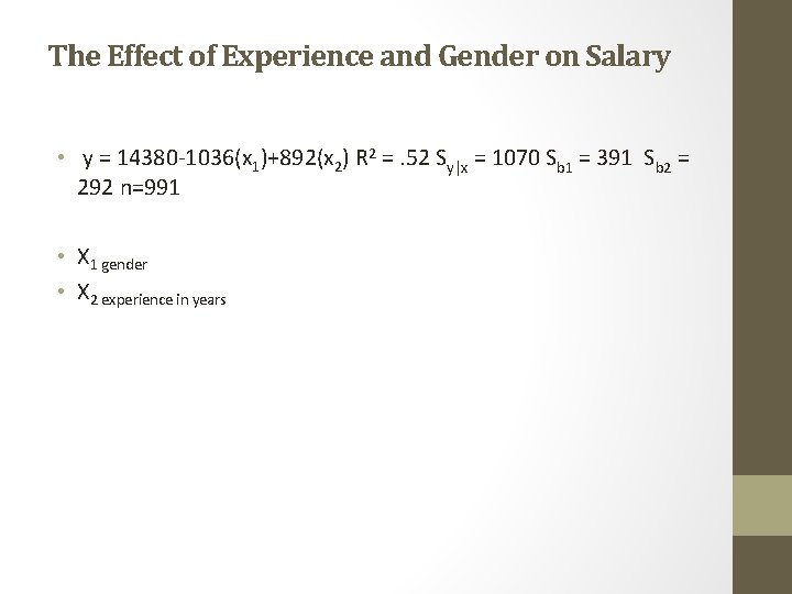
The Effect of Experience and Gender on Salary • y = 14380 -1036(x 1)+892(x 2) R 2 =. 52 Sy|x = 1070 Sb 1 = 391 Sb 2 = 292 n=991 • X 1 gender • X 2 experience in years

Interpretation of Multivariate Regression Equation • Intercept • The intercept is the value of the dependent variable when all the independent variables are equal to 0. • In this case, the regression line predicts someone to earn $14, 380 if they are a male and have no experience.

Interpretation of Multivariate Regression Equation • The slopes • We now have two slopes. The slope is interpreted as the change in the dependent variable associated with a one unit change in the independent variable, holding the other independent variables constant. • “Holding a variable constant” means that its value does not change while the value of the other independent variable changes. In multivariate regression the slopes are called partial slopes, partial regression coefficients.

Interpretation of Multivariate Regression Equation • Gender Slope X 1 • In our above example we observe that women earn $1, 036 less than men, holding experience constant. • Experience Slope X 2 • An additional year of experience is associated with an $892 increase in salary, holding gender constant. • The fact that we can “hold constant” the other independent variables makes multivariate regression an extremely powerful tool.

Interpretation • R 2 is interpreted as before, but it now represents the amount of variation in X determined by both independent variables. We say that gender and experience together explain 52% of the variation in salary. • The Standard Error of the Estimate Sy|x • We can again use Sy|x to approximate confidence intervals around our predictions of Y at the mean value of X. In this case the standard error of the estimate is 1070.

Interpretation • Inference and Hypothesis testing • We use the standard error for each slope to construct confidence intervals about each slope. We also use each slope’s respective standard error to test the hypothesis that the true slope is equal to 0. The d. f. is n-k-1 where n is the sample size and k is the number of independent variables.

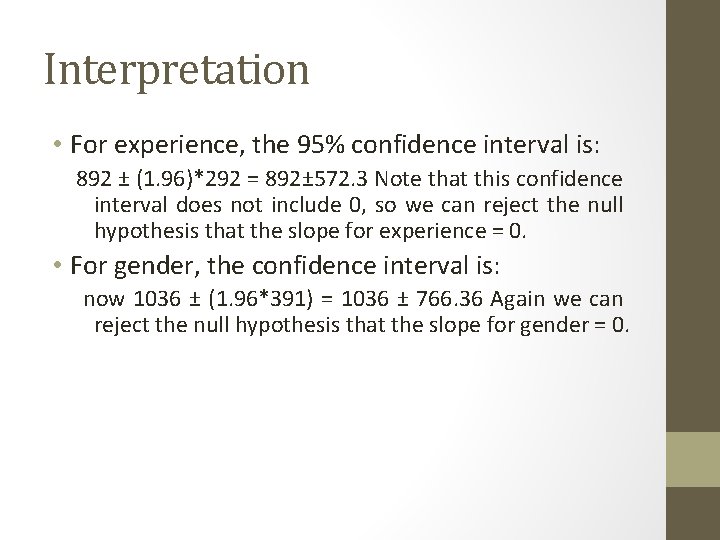
Interpretation • For experience, the 95% confidence interval is: 892 ± (1. 96)*292 = 892± 572. 3 Note that this confidence interval does not include 0, so we can reject the null hypothesis that the slope for experience = 0. • For gender, the confidence interval is: now 1036 ± (1. 96*391) = 1036 ± 766. 36 Again we can reject the null hypothesis that the slope for gender = 0.

Interpretation • What can we say to the judge about Acme’s claim that women are not discriminated against but receive lower salaries because they have less experience?

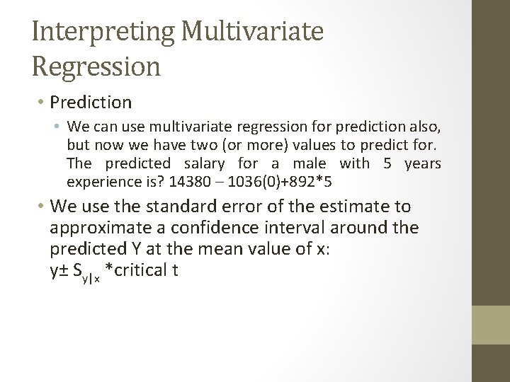
Interpreting Multivariate Regression • Prediction • We can use multivariate regression for prediction also, but now we have two (or more) values to predict for. The predicted salary for a male with 5 years experience is? 14380 – 1036(0)+892*5 • We use the standard error of the estimate to approximate a confidence interval around the predicted Y at the mean value of x: y± Sy|x *critical t

F statistic • The F-Ratio – an additional measure of statistical significance • The F-ratio tells us whether the regression equation as a whole is statistically significant from 0. • Intuitively, it is the ratio of the amount of variation explained by the model to the amount of variation unexplained by the model observed due to chance • Explained Sum of Squares/Residual Sum of Squares • With the number of independent variables minus 1 as the df in the numerator, and the sample size minus the number of independent variables as the df in the denominator

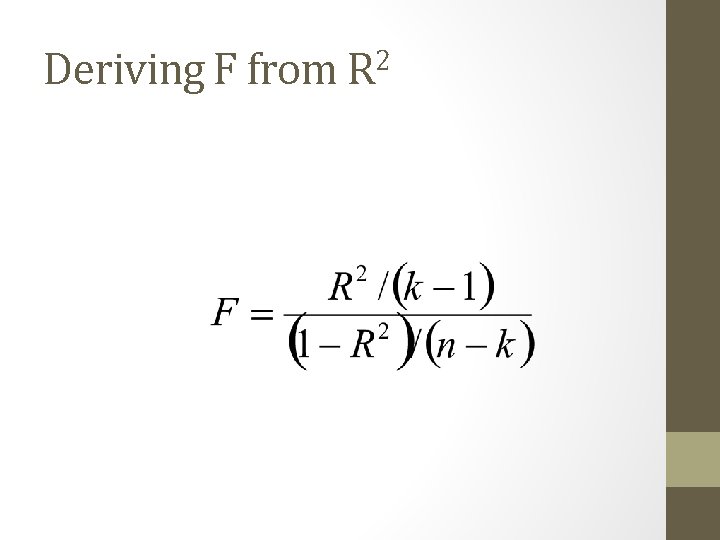
Deriving F from R 2

The F statistic • Where k = the number of independent variables • N = the sample size • Use the f statistic to test whether all the slopes are simultaneously equal to 0

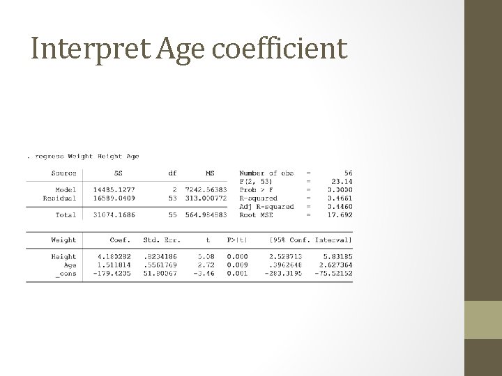
Examples • Weight and Height model from previous class • Form a hypothesis about adding age to the model • What is your null hypothesis?

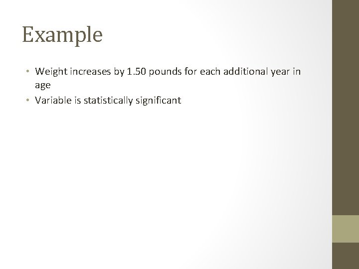
Interpret Age coefficient

Example • Weight increases by 1. 50 pounds for each additional year in age • Variable is statistically significant

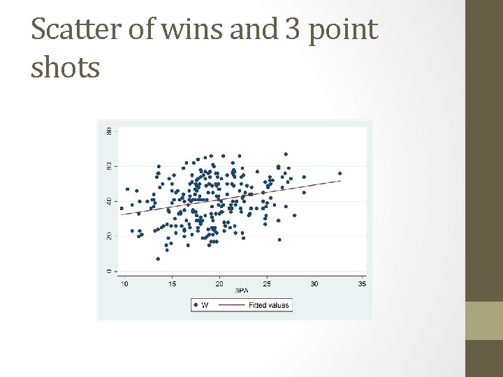
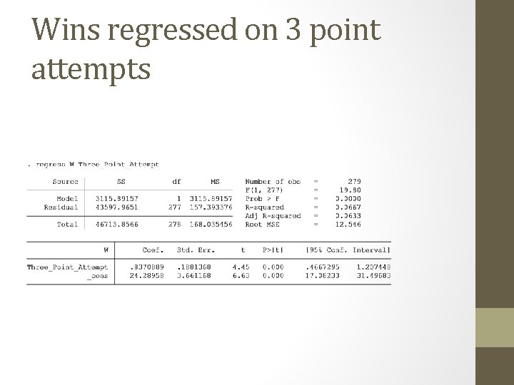
Example NBA season started last week • Do teams that take a lot of three point shots win more games? • Regress number of wins in a season on the average number of 3 point shots taken per game • Data taken from 2006 -2015 seasons

Scatter of wins and 3 point shots

Wins regressed on 3 point attempts

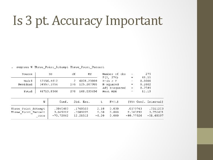
Is 3 pt. Accuracy Important • Anyone can take 3 point shots • Perhaps accuracy is most important?

Is 3 pt. Accuracy Important

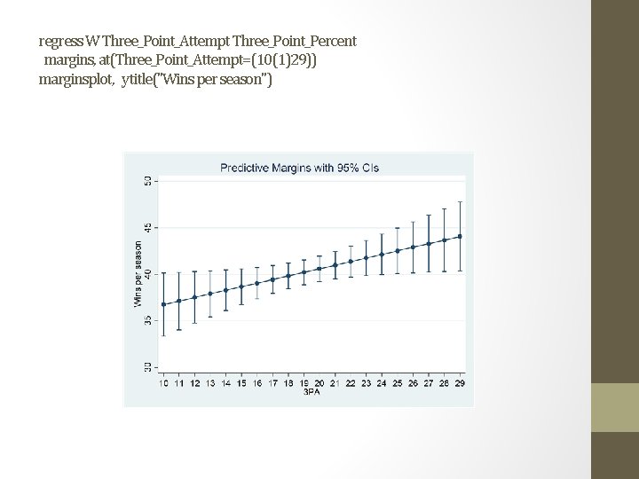
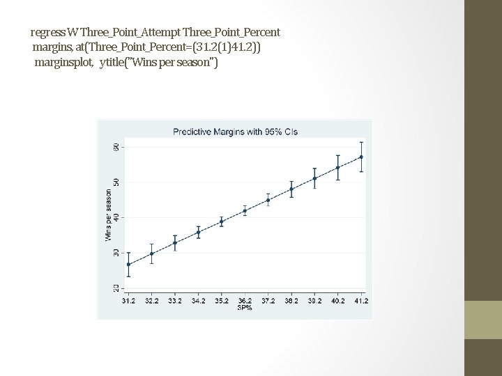
What would you tell a General Manager devising a strategy to win NBA games?

regress W Three_Point_Attempt Three_Point_Percent margins, at(Three_Point_Attempt=(10(1)29)) marginsplot, ytitle("Wins per season")

regress W Three_Point_Attempt Three_Point_Percent margins, at(Three_Point_Percent=(31. 2(1)41. 2)) marginsplot, ytitle("Wins per season")

Evaluating Independent Variables • How important is each additional independent variable • Metrics • • • Theoretical importance Statistical significance Substantive importance Standardized Betas Partitioning variance

Evaluating Independent Variables • How important is each additional independent variable • Metrics • Theoretical importance • If theory is well developed this may be the most important criteria for deciding whether to include a variable • If theory is uncertain and you are testing a hypothesis attach more weight to statistical tests

Evaluating Independent Variables • How important is each additional independent variable • Metrics • Substantive importance • How meaningful is the result? Interpretation here is based on substantive knowledge of topic

Evaluating Independent Variables • How important is each additional independent variable • Metrics • Statistical significance • Is the slope statistically significant from zero? • Beware the Statistical Significance Trap • Or Type 1 error • With a 95% level of confidence 1 out of 20 times we expect to make a type 1 error

Evaluating Independent Variables • Example • I added height and weights from a prior class to the height weight data • Using the height weight data I asked Stata to generate a random variable • Each of the student has a number randomly generated associated with your height and weight

Evaluating Independent Variables • Example • Develop a hypothesis about the effect of the random variable on your weight • Do you expect this hypothesis to be correct? Why? • Do you have an expectation about the sign (i. e. negative or positive)? • Compared to a model with only height as an independent variable will adding this variable change the R 2

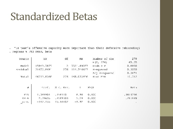
Evaluating Independent Variables • How important is each additional independent variable • Metrics • Standardized Betas • Are three point shots attempted more important than free throws attempted? • Measured in similar units, did the player take a shot?

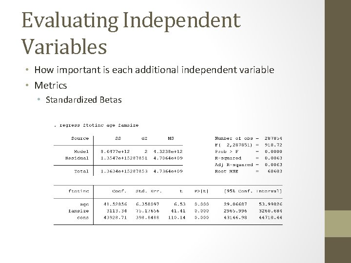
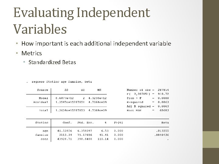
Evaluating Independent Variables • How important is each additional independent variable • Metrics • Standardized Betas • Is age more important than family size in determining income? • Measured in different units

Evaluating Independent Variables • How important is each additional independent variable • Metrics • Standardized Betas

Evaluating Independent Variables • How important is each additional independent variable • Metrics • Standardized Betas

Evaluating Independent Variables • How important is each additional independent variable • Metrics • Standardized Betas • Measured in different units • Standardized betas measure coefficients in terms of standard deviations • Interpretation: How many standard deviations will the dependent variable change for a one standard deviation change in the independent variable

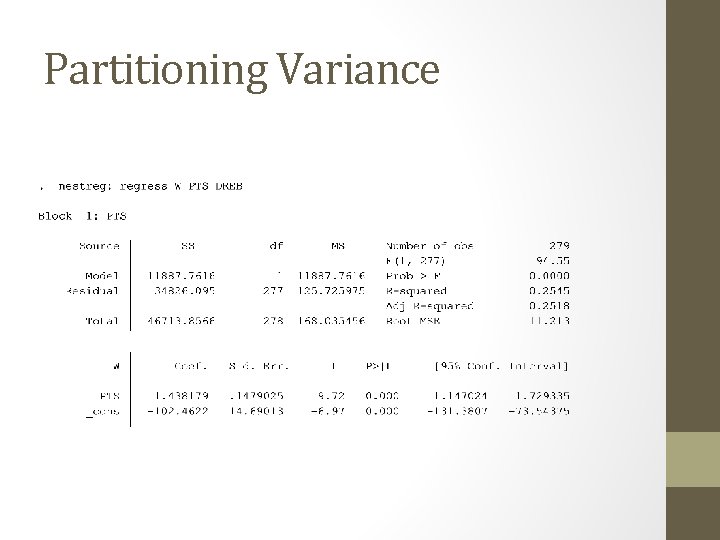
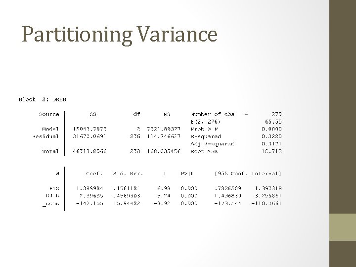
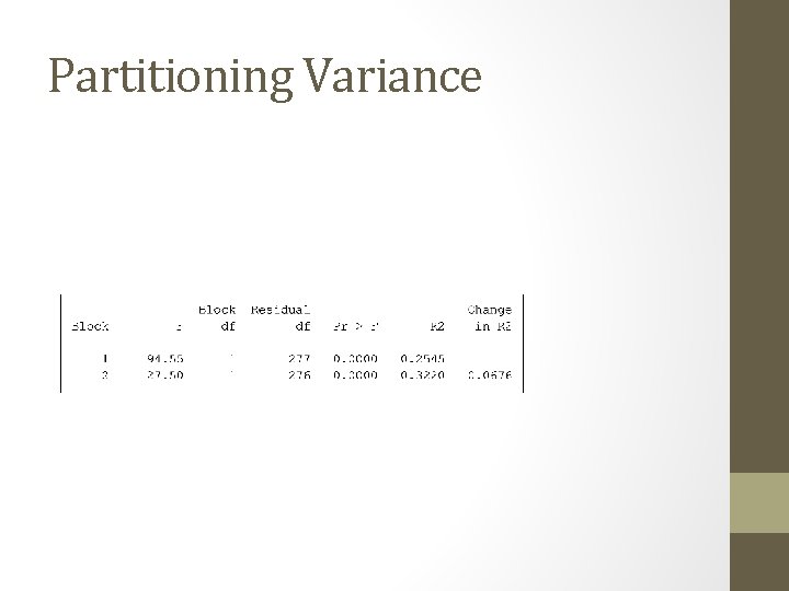
Evaluating Independent Variables • How important is each additional independent variable • Metrics • Partitioning variance • R 2 how much variance by independent variables • How much additional variance is explained by the addition of an independent variable

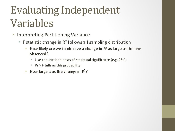
Evaluating Independent Variables • Interpreting Partitioning Variance • F statistic change in R 2 follows a f sampling distribution • How likely are we to observe a change in R 2 as large as the one observed? • Use conventional tests of statistical significance (e. g. 95%) • Pr > F tells us this probability • How large was the change in R 2?

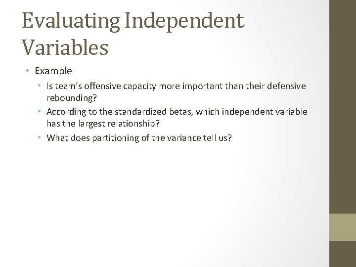
Evaluating Independent Variables • Example • Is team’s offensive capacity more important than their defensive rebounding? • According to the standardized betas, which independent variable has the largest relationship? • What does partitioning of the variance tell us?

Standardized Betas

Partitioning Variance

Partitioning Variance

Partitioning Variance

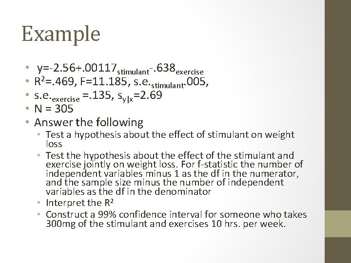
Example • A researcher wants to know the effects of exercise and using a stimulant on weight loss. Four levels of exercise(hrs. per week) and four levels of the stimulant(mg/day) are used. She conducts an experiment on 24 college students. Weight loss in pounds is the dependent variable. The following results are obtained

Example • • • y=-2. 56+. 00117 stimulant-. 638 exercise R 2=. 469, F=11. 185, s. e. stimulant. 005, s. e. exercise =. 135, sy|x=2. 69 N = 305 Answer the following • Test a hypothesis about the effect of stimulant on weight loss • Test the hypothesis about the effect of the stimulant and exercise jointly on weight loss. For f-statistic the number of independent variables minus 1 as the df in the numerator, and the sample size minus the number of independent variables as the df in the denominator • Interpret the R 2 • Construct a 99% confidence interval for someone who takes 300 mg of the stimulant and exercises 10 hrs. per week.

Some differences between multivariate and bivariate regression • When we add another variable to a regression equation the R 2 almost certainly increases. • Most software will produce an adjusted R 2 that takes this into consideration and provides a lower value for R 2 Use the adjusted value in practice • 2. Adding another variable may change the slope of the 1 st independent variable. • The F-statistic is used in multivariate regression for inference

Multicollinearity • Multicollinearity is the degree to which the independent variables in a multivariate regression equation are related to each other. Thus, multicollinearity can be thought of as a continuum. • Problem: Perfect multicollinearity exists when one independent variable is a direct linear function of another.

Multicollinearity • More common is high multicollinearity. High multicollinearity means the independent variables are highly correlated with each other. • With perfect multicollinearity you cannot estimate an OLS equation. With high multicollinearity, a regression equation can be estimated, but the standard errors will be inflated. Consequently, it will be difficult for any of the slopes to achieve statistical significance.

Detecting multicollinearity • In the presence of perfect multiocollinearity, an OLS equation cannot be estimated. • Consequently, you will certainly be aware of a situation where you have perfect multicollinearity. This is typically a sign of a data error such as assigning the same number of variables as categories for a dummy variable. • Theory. Detecting high multicollinearity is a little trickier. As always, theory can be a good start. If two independent variables appear to be conceptually related to one another, you should be suspicious of possible multicollinearity.

Detecting multicollinearity • For example, if you regressed a student’s undergraduate GPA on their math SAT and verbal SAT using two independent variables to represent each score, respectively, multicollinearity could be a potential problem. A student’s math SAT and verbal SAT are likely to be highly correlated. • High R 2 but none or most of the independent variables are statistically significant. • This is usually a sign of multicollinearity. This occurs because the independent variables together explain much of the variation in Y, but because the independent variables are highly correlated, we cannot partition the explained variation to either of the independent variables.

Detecting multicollinearity • Regress each independent variable on all other independent variables. • This is the most rigorous and consequently the preferred method for detecting high multicollinearity. • When the R 2 from any of these equations is close to 1. 0, there is a high degree of multicollinearity.

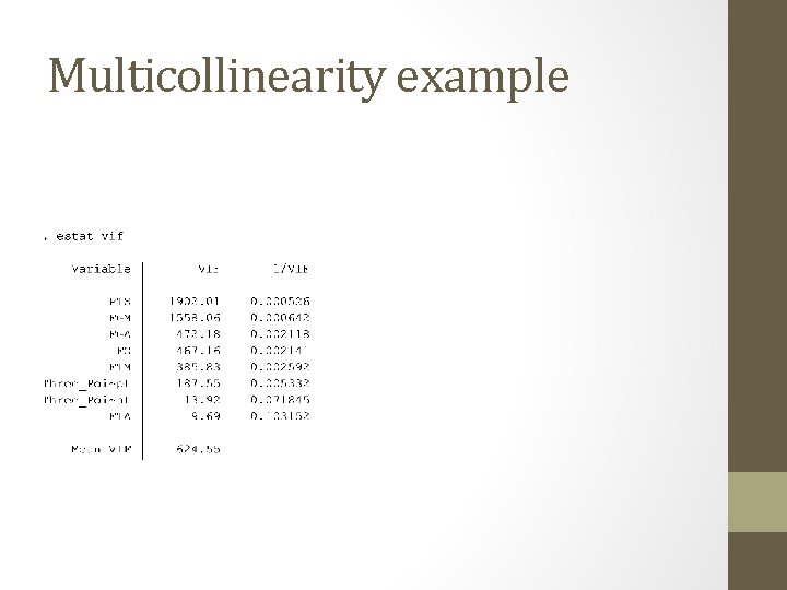
Detecting multicollinearity • Regress each independent variable on all other independent variables. • Stata: use “estat vif “ • 1/vif column = 1 – R 2

Multicollinearity Example

Multicollinearity example

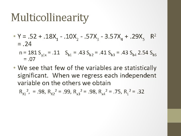
Multicollinearity • An example of high multicollinearity: • The sociologist Gino Germani wants to explain varying levels of voter support in Argentine counties former President Juan Peron in the 1946 elections. Germani reasons that percentage of a county’s presidential support going to Peron is determined by: • the % of workers in a county who are blue collar (X 1), the percentage of workers in a county who are farmers (X 2), the percentage of workers in a county who are white collar (X 3), and the % of the population born outside the county. Germani uses OLS to estimate the regression equation and obtains:

Multicollinearity • Y =. 52 +. 18 X 1 -. 10 X 2 -. 57 X 3 - 3. 57 X 4 +. 29 X 5 R 2 =. 24 n = 181 Sy|x =. 11 Sb 1 =. 43 Sb 2 =. 41 Sb 3 =. 43 Sb 4 2. 54 Sb 5 =. 07 • We see that few of the variables are statistically significant. When we regress each independent variable on the others we obtain RX 12, =. 98, RX 22 =. 99, Rx 32 =. 98, Rx 42 =. 75, R 12 =. 32

An example of Multicollinearity • Clearly, we have a problem with multicollinearity. The high R 2 s when using the first 3 independent variables as dependent variables tips us off. This is not surprising because 3 of the independent variables reflect very similar concepts.

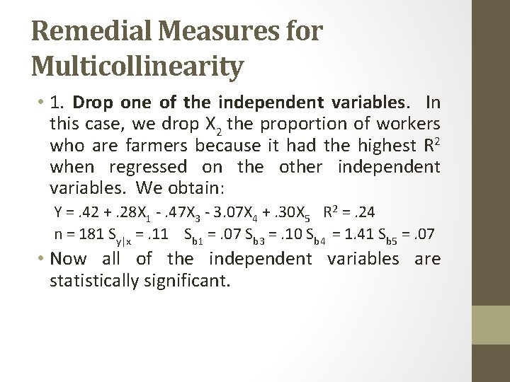
Remedial Measures for Multicollinearity • 1. Drop one of the independent variables. In this case, we drop X 2 the proportion of workers who are farmers because it had the highest R 2 when regressed on the other independent variables. We obtain: Y =. 42 +. 28 X 1 -. 47 X 3 - 3. 07 X 4 +. 30 X 5 R 2 =. 24 n = 181 Sy|x =. 11 Sb 1 =. 07 Sb 3 =. 10 Sb 4 = 1. 41 Sb 5 =. 07 • Now all of the independent variables are statistically significant.

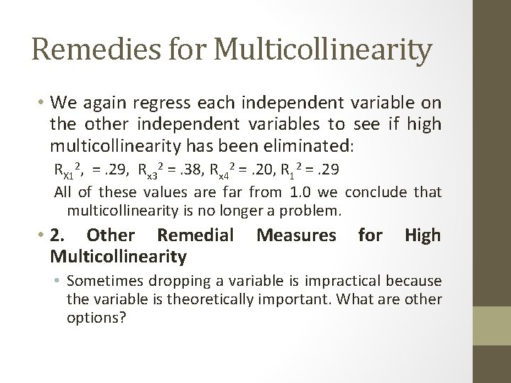
Remedies for Multicollinearity • We again regress each independent variable on the other independent variables to see if high multicollinearity has been eliminated: RX 12, =. 29, Rx 32 =. 38, Rx 42 =. 20, R 12 =. 29 All of these values are far from 1. 0 we conclude that multicollinearity is no longer a problem. • 2. Other Remedial Multicollinearity Measures for High • Sometimes dropping a variable is impractical because the variable is theoretically important. What are other options?

Remedies for Multicollinearity • A. Increase the sample size. The major problem with multicollinearity is that it makes it difficult for the slopes of the independent variables to achieve statistical significance. But recall that increasing the sample size makes it easier to achieve statistical significance. • B. Combine two variables into one. Sometimes a composite variable can be created from two others that are closely related.

When to use Regression If the dependent variable is an interval level variable, and you want to assess its relationship with another variable, OLS regression is a good tool to use. It is generally more powerful than the other statistical techniques we have learned thus far.

Uses of Regression • Regression tells us: • • If a relationship exists between two variables (Is the slope = to 0) Predictive power of the association (R 2) The strength of the relationship (size of slope) Allows for prediction (insert values into x)