Multiple Linear Regression Multiple Regression In multiple regression

- Slides: 46

Multiple Linear Regression

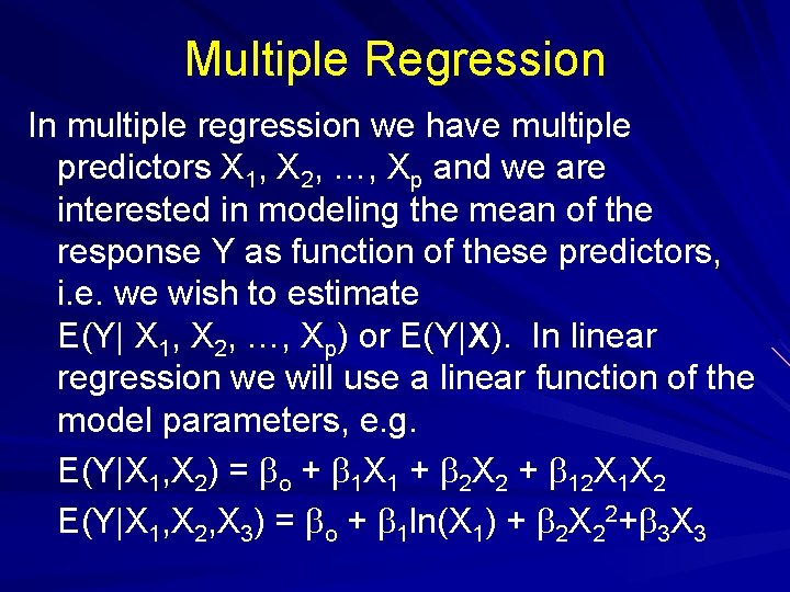
Multiple Regression In multiple regression we have multiple predictors X 1, X 2, …, Xp and we are interested in modeling the mean of the response Y as function of these predictors, i. e. we wish to estimate E(Y| X 1, X 2, …, Xp) or E(Y|X). In linear regression we will use a linear function of the model parameters, e. g. E(Y|X 1, X 2) = bo + b 1 X 1 + b 2 X 2 + b 12 X 1 X 2 E(Y|X 1, X 2, X 3) = bo + b 1 ln(X 1) + b 2 X 22+b 3 X 3

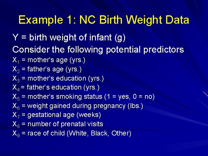
Example 1: NC Birth Weight Data Y = birth weight of infant (g) Consider the following potential predictors X 1 = mother’s age (yrs. ) X 2 = father’s age (yrs. ) X 3 = mother’s education (yrs. ) X 4 = father’s education (yrs. ) X 5 = mother’s smoking status (1 = yes, 0 = no) X 6 = weight gained during pregnancy (lbs. ) X 7 = gestational age (weeks) X 8 = number of prenatal visits X 9 = race of child (White, Black, Other)

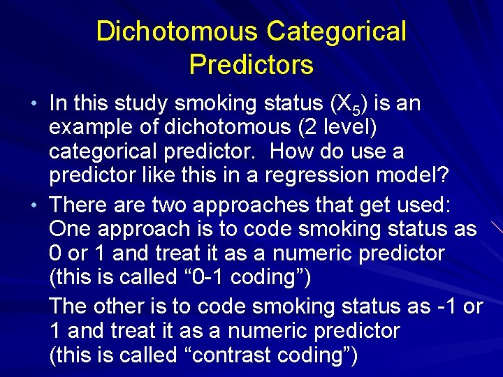
Dichotomous Categorical Predictors • In this study smoking status (X 5) is an example of dichotomous (2 level) categorical predictor. How do use a predictor like this in a regression model? • There are two approaches that get used: One approach is to code smoking status as 0 or 1 and treat it as a numeric predictor (this is called “ 0 -1 coding”) The other is to code smoking status as -1 or 1 and treat it as a numeric predictor (this is called “contrast coding”)

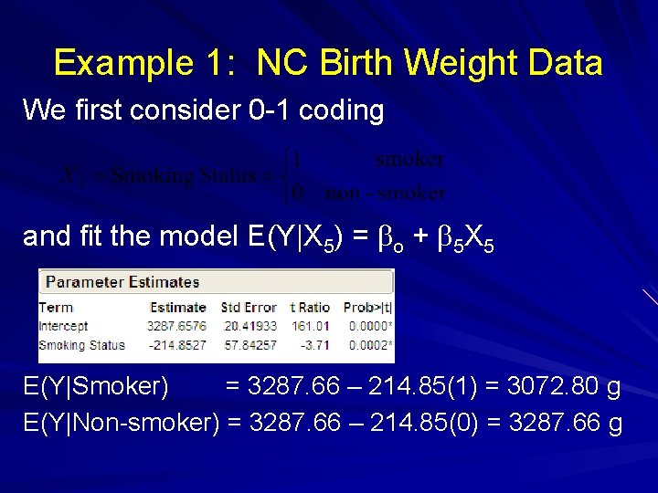
Example 1: NC Birth Weight Data We first consider 0 -1 coding and fit the model E(Y|X 5) = bo + b 5 X 5 E(Y|Smoker) = 3287. 66 – 214. 85(1) = 3072. 80 g E(Y|Non-smoker) = 3287. 66 – 214. 85(0) = 3287. 66 g

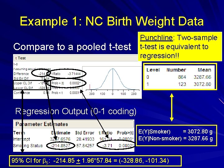
Example 1: NC Birth Weight Data Compare to a pooled t-test Punchline: Two-sample t-test is equivalent to regression!! Regression Output (0 -1 coding) E(Y|Smoker) = 3072. 80 g E(Y|Non-smoker) = 3287. 66 g 95% CI for b 5: -214. 85 + 1. 96*57. 84 = (-328. 86, -101. 34)

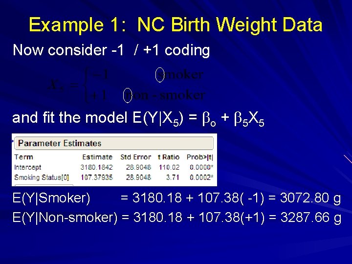
Example 1: NC Birth Weight Data Now consider -1 / +1 coding and fit the model E(Y|X 5) = bo + b 5 X 5 E(Y|Smoker) = 3180. 18 + 107. 38( -1) = 3072. 80 g E(Y|Non-smoker) = 3180. 18 + 107. 38(+1) = 3287. 66 g

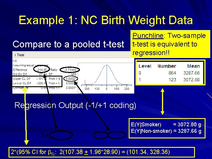
Example 1: NC Birth Weight Data Compare to a pooled t-test Punchline: Two-sample t-test is equivalent to regression!! Regression Output (-1/+1 coding) 2 x E(Y|Smoker) = 3072. 80 g E(Y|Non-smoker) = 3287. 66 g 2*(95% CI for b 5): 2(107. 38 + 1. 96*28. 90) = (101. 34, 328. 36)

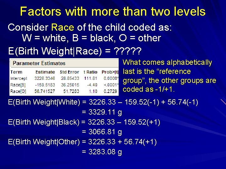
Factors with more than two levels Consider Race of the child coded as: W = white, B = black, O = other E(Birth Weight|Race) = ? ? ? What comes alphabetically last is the “reference group”, the other groups are coded as -1/+1. E(Birth Weight|White) = 3226. 33 – 159. 52(-1) + 56. 74(-1) = 3329. 11 g E(Birth Weight|Black) = 3226. 33 – 159. 52(+1) = 3066. 81 g E(Birth Weight|Other) = 3226. 33 + 56. 74(+1) = 3283. 08 g

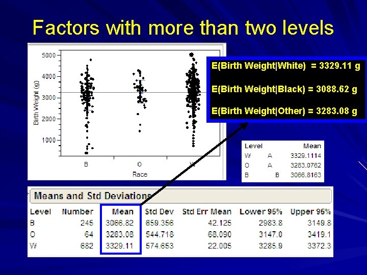
Factors with more than two levels E(Birth Weight|White) = 3329. 11 g E(Birth Weight|Black) = 3088. 62 g E(Birth Weight|Other) = 3283. 08 g

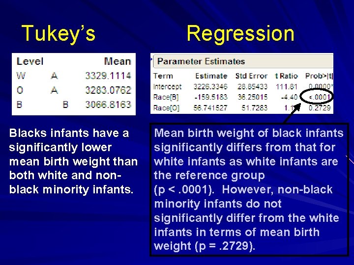
Tukey’s Blacks infants have a significantly lower mean birth weight than both white and nonblack minority infants. Regression Mean birth weight of black infants significantly differs from that for white infants as white infants are the reference group (p <. 0001). However, non-black minority infants do not significantly differ from the white infants in terms of mean birth weight (p =. 2729).

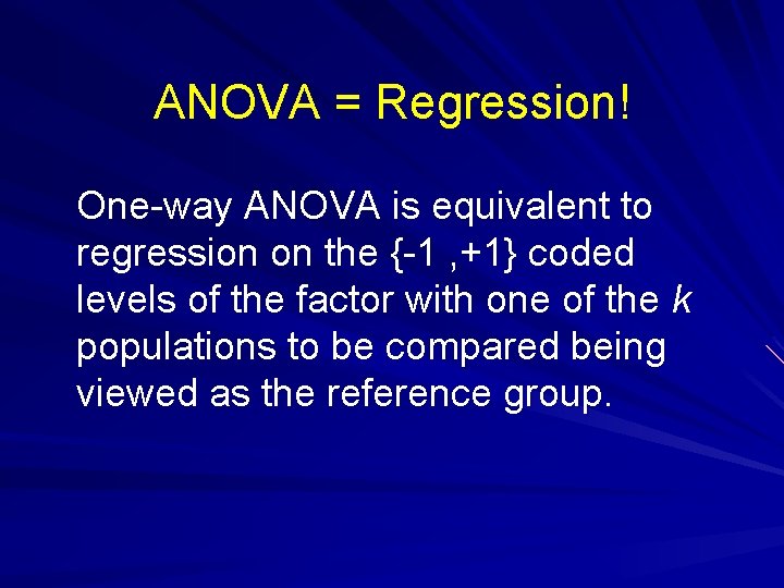
ANOVA = Regression! One-way ANOVA is equivalent to regression on the {-1 , +1} coded levels of the factor with one of the k populations to be compared being viewed as the reference group.

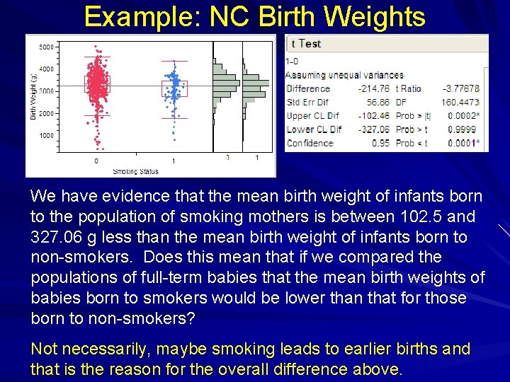
Example: NC Birth Weights We have evidence that the mean birth weight of infants born to the population of smoking mothers is between 102. 5 and 327. 06 g less than the mean birth weight of infants born to non-smokers. Does this mean that if we compared the populations of full-term babies that the mean birth weights of babies born to smokers would be lower than that for those born to non-smokers? Not necessarily, maybe smoking leads to earlier births and that is the reason for the overall difference above.

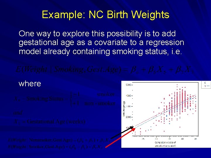
Example: NC Birth Weights One way to explore this possibility is to add gestational age as a covariate to a regression model already containing smoking status, i. e. where

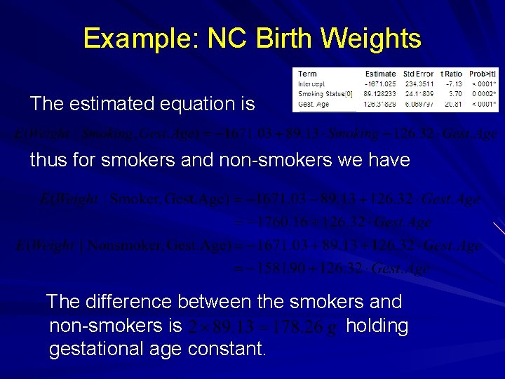
Example: NC Birth Weights The estimated equation is thus for smokers and non-smokers we have The difference between the smokers and non-smokers is holding gestational age constant.

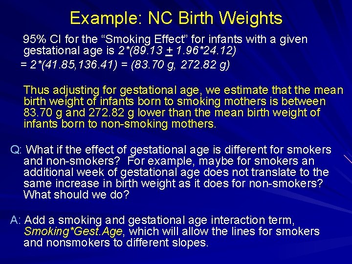
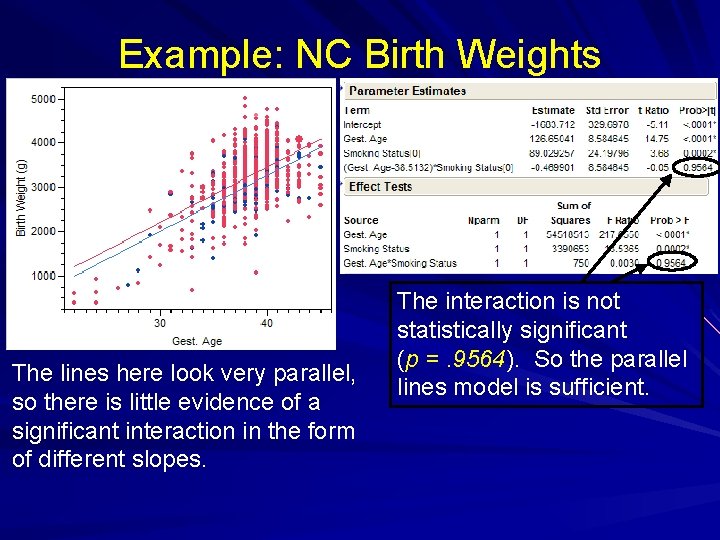
Example: NC Birth Weights 95% CI for the “Smoking Effect” for infants with a given gestational age is 2*(89. 13 + 1. 96*24. 12) = 2*(41. 85, 136. 41) = (83. 70 g, 272. 82 g) Thus adjusting for gestational age, we estimate that the mean birth weight of infants born to smoking mothers is between 83. 70 g and 272. 82 g lower than the mean birth weight of infants born to non-smoking mothers. Q: What if the effect of gestational age is different for smokers and non-smokers? For example, maybe for smokers an additional week of gestational age does not translate to the same increase in birth weight as it does for non-smokers? What should we do? A: Add a smoking and gestational age interaction term, Smoking*Gest. Age, which will allow the lines for smokers and nonsmokers to different slopes.

Example: NC Birth Weights The lines here look very parallel, so there is little evidence of a significant interaction in the form of different slopes. The interaction is not statistically significant (p =. 9564). So the parallel lines model is sufficient.

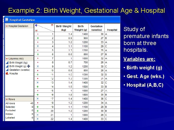
Example 2: Birth Weight, Gestational Age & Hospital Study of premature infants born at three hospitals. Variables are: • Birth weight (g) • Gest. Age (wks. ) • Hospital (A, B, C)

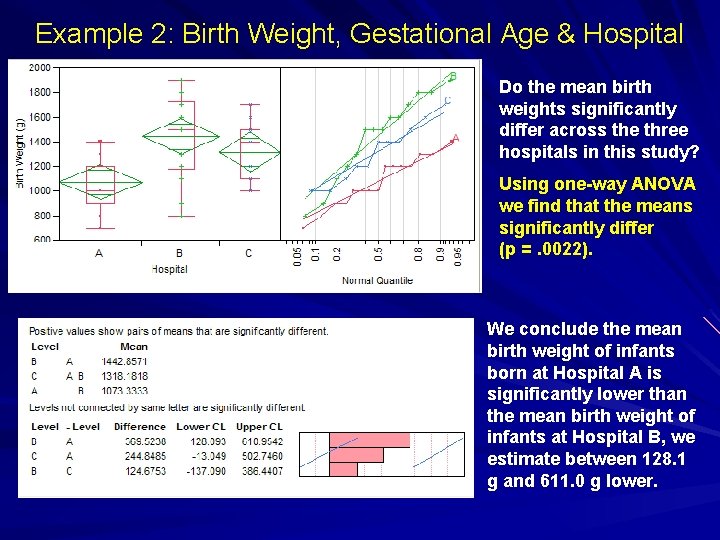
Example 2: Birth Weight, Gestational Age & Hospital Do the mean birth weights significantly differ across the three hospitals in this study? Using one-way ANOVA we find that the means significantly differ (p =. 0022). We conclude the mean birth weight of infants born at Hospital A is significantly lower than the mean birth weight of infants at Hospital B, we estimate between 128. 1 g and 611. 0 g lower.

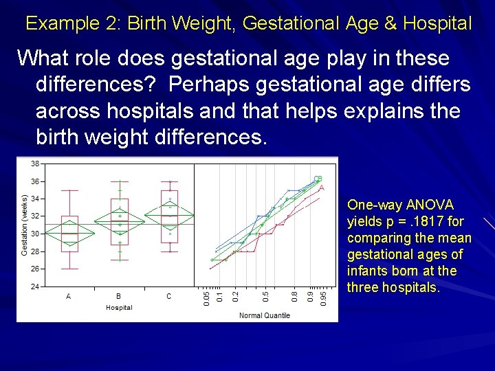
Example 2: Birth Weight, Gestational Age & Hospital What role does gestational age play in these differences? Perhaps gestational age differs across hospitals and that helps explains the birth weight differences. One-way ANOVA yields p =. 1817 for comparing the mean gestational ages of infants born at the three hospitals.

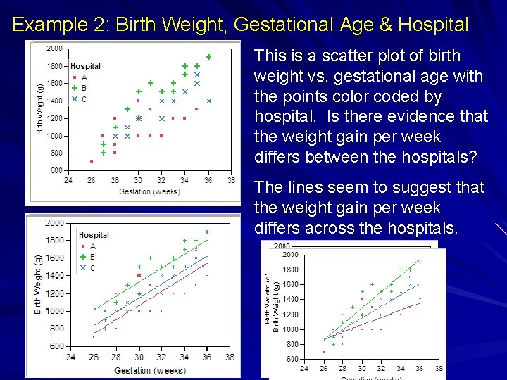
Example 2: Birth Weight, Gestational Age & Hospital This is a scatter plot of birth weight vs. gestational age with the points color coded by hospital. Is there evidence that the weight gain per week differs between the hospitals? The lines seem to suggest that the weight gain per week differs across the hospitals.

Example 2: Birth Weight, Gestational Age & Hospital

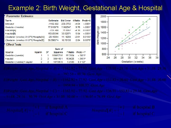
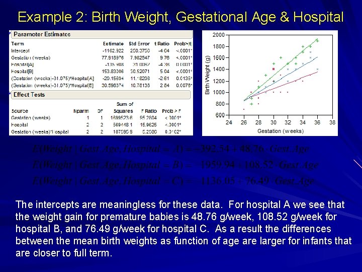
Example 2: Birth Weight, Gestational Age & Hospital The intercepts are meaningless for these data. For hospital A we see that the weight gain for premature babies is 48. 76 g/week, 108. 52 g/week for hospital B, and 76. 49 g/week for hospital C. As a result the differences between the mean birth weights as function of age are larger for infants that are closer to full term.

Analysis of Covariance (ANCOVA) These two examples are analysis of covariance models where we were primarily interested in potential differences between populations defined but a nominal variable (e. g. smoking status) and we are making adjustment in that comparison for other factors such as gestational age. The variables that we are adjusting for are called covariates.

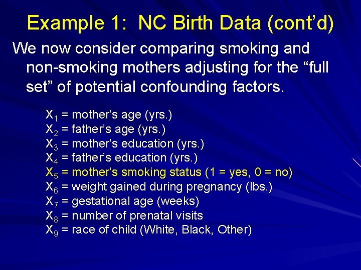
Example 1: NC Birth Data (cont’d) We now consider comparing smoking and non-smoking mothers adjusting for the “full set” of potential confounding factors. X 1 = mother’s age (yrs. ) X 2 = father’s age (yrs. ) X 3 = mother’s education (yrs. ) X 4 = father’s education (yrs. ) X 5 = mother’s smoking status (1 = yes, 0 = no) X 6 = weight gained during pregnancy (lbs. ) X 7 = gestational age (weeks) X 8 = number of prenatal visits X 9 = race of child (White, Black, Other)

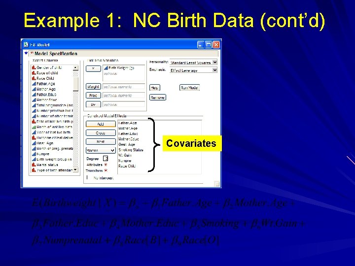
Example 1: NC Birth Data (cont’d) Covariates

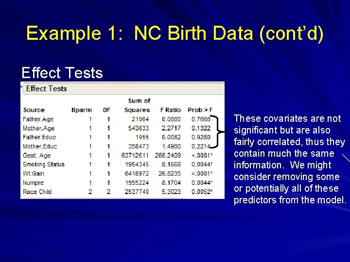
Example 1: NC Birth Data (cont’d) Effect Tests These covariates are not significant but are also fairly correlated, thus they contain much the same information. We might consider removing some or potentially all of these predictors from the model.

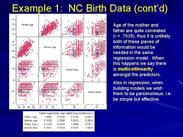
Example 1: NC Birth Data (cont’d) Age of the mother and father are quite correlated (r =. 7539), thus it is unlikely both of these pieces of information would be needed in the same regression model. When this happens we say there is multicollinearity amongst the predictors. Also in regression, when building models we wish them to be parsimonious, i. e. be simple but effective.

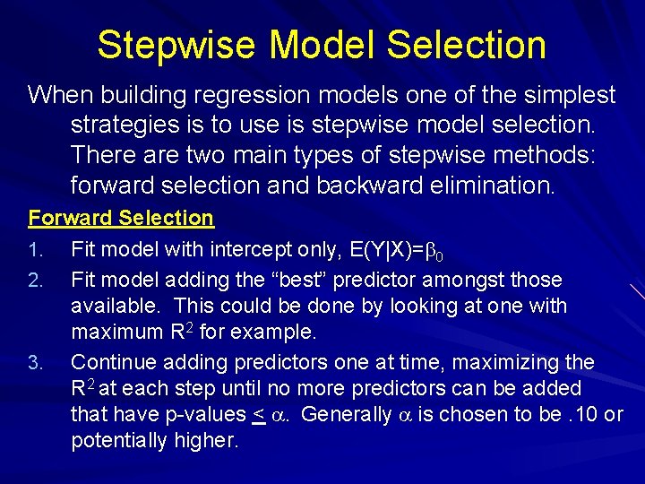
Stepwise Model Selection When building regression models one of the simplest strategies is to use is stepwise model selection. There are two main types of stepwise methods: forward selection and backward elimination. Forward Selection 1. Fit model with intercept only, E(Y|X)=b 0 2. Fit model adding the “best” predictor amongst those available. This could be done by looking at one with maximum R 2 for example. 3. Continue adding predictors one at time, maximizing the R 2 at each step until no more predictors can be added that have p-values < a. Generally a is chosen to be. 10 or potentially higher.

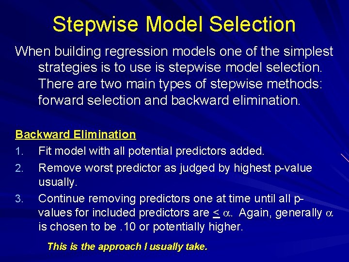
Stepwise Model Selection When building regression models one of the simplest strategies is to use is stepwise model selection. There are two main types of stepwise methods: forward selection and backward elimination. Backward Elimination 1. Fit model with all potential predictors added. 2. Remove worst predictor as judged by highest p-value usually. 3. Continue removing predictors one at time until all pvalues for included predictors are < a. Again, generally a is chosen to be. 10 or potentially higher. This is the approach I usually take.

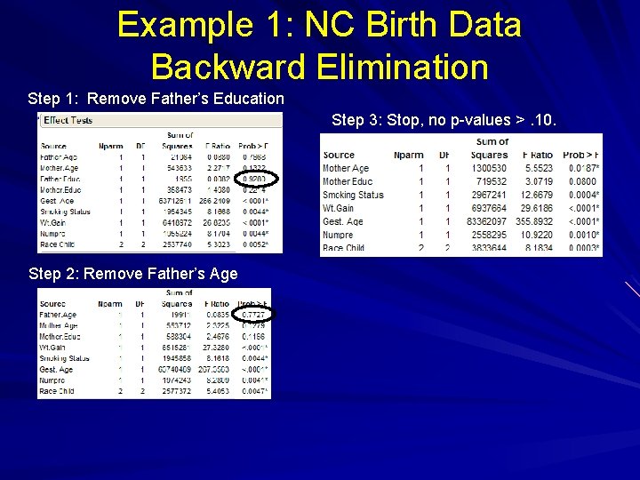
Example 1: NC Birth Data Backward Elimination Step 1: Remove Father’s Education Step 3: Stop, no p-values >. 10. Step 2: Remove Father’s Age

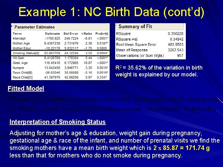
Example 1: NC Birth Data (cont’d) R 2 = 35. 62% of the variation in birth weight is explained by our model. Fitted Model Interpretation of Smoking Status Adjusting for mother’s age & education, weight gain during pregnancy, gestational age & race of the infant, and number of prenatal visits we find the smoking mothers have a mean birth weight which is 2 x 85. 87 = 171. 74 g less than that for mothers who do not smoke during pregnancy.

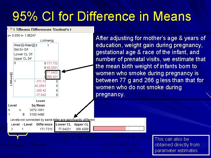
95% CI for Difference in Means After adjusting for mother’s age & years of education, weight gain during pregnancy, gestational age & race of the infant, and number of prenatal visits, we estimate that the mean birth weight of infants born to women who smoke during pregnancy is between 77 g and 266 g less than that for women who do not smoke during pregnancy. This can also be obtained directly from parameter estimates.

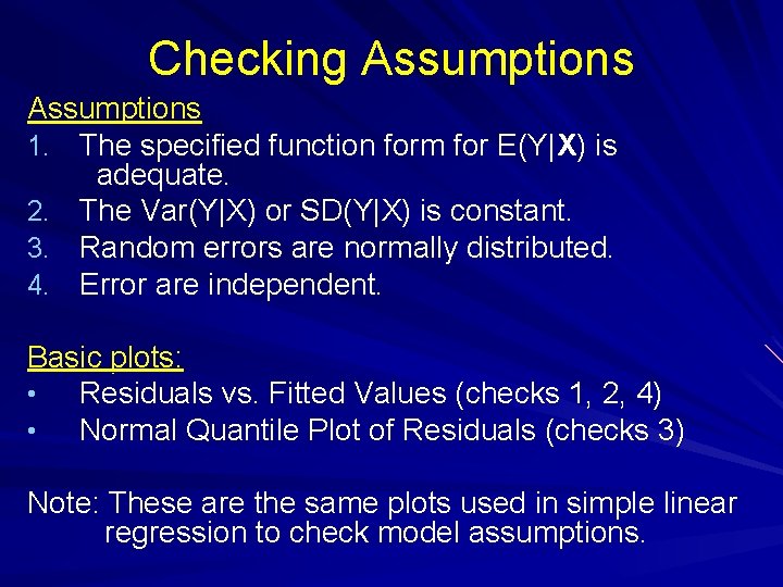
Checking Assumptions 1. The specified function form for E(Y|X) is adequate. 2. The Var(Y|X) or SD(Y|X) is constant. 3. Random errors are normally distributed. 4. Error are independent. Basic plots: • Residuals vs. Fitted Values (checks 1, 2, 4) • Normal Quantile Plot of Residuals (checks 3) Note: These are the same plots used in simple linear regression to check model assumptions.

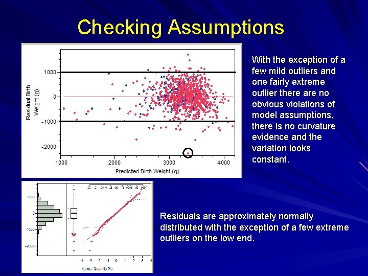
Checking Assumptions With the exception of a few mild outliers and one fairly extreme outlier there are no obvious violations of model assumptions, there is no curvature evidence and the variation looks constant. Residuals are approximately normally distributed with the exception of a few extreme outliers on the low end.

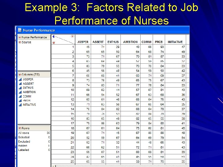
Example 3: Factors Related to Job Performance of Nurses A nursing director would like to use nurses’ personal characteristics to develop a regression model for predicting job performance (JOBPER). The following potential predictors are available: • • X 1 = assertiveness (ASSERT) X 2 = enthusiasm (ENTHUS) X 3 = ambition (AMBITION) X 4 = communication skills (COMM) X 5 = problem-solving skills (PROB) X 6 = initiative (INITIATIVE) Y = job performance (JOBPER)

Example 3: Factors Related to Job Performance of Nurses

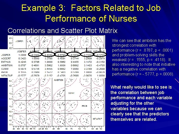
Example 3: Factors Related to Job Performance of Nurses Correlations and Scatter Plot Matrix We can see that ambition has the strongest correlation with performance (r =. 8787, p <. 0001) and problem-solving skills the weakest (r =. 1555, p =. 4118). It also interesting to note that initiative has a negative correlation with performance (r = -. 5777, p =. 0008). What really would like to see is the correlation between job performance and each variable adjusting for the other variables because we can clearly see that the predictors themselves are related.

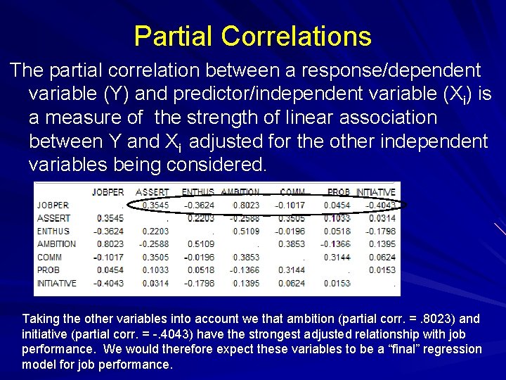
Partial Correlations The partial correlation between a response/dependent variable (Y) and predictor/independent variable (Xi) is a measure of the strength of linear association between Y and Xi adjusted for the other independent variables being considered. Taking the other variables into account we that ambition (partial corr. =. 8023) and initiative (partial corr. = -. 4043) have the strongest adjusted relationship with job performance. We would therefore expect these variables to be a “final” regression model for job performance.

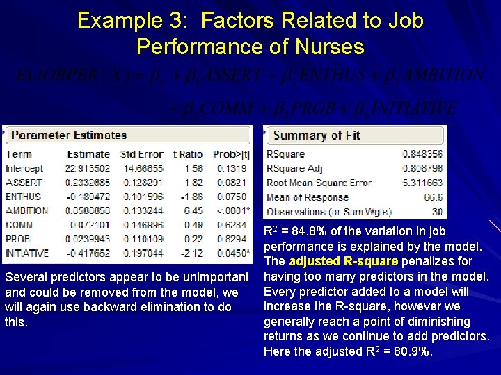
Example 3: Factors Related to Job Performance of Nurses Several predictors appear to be unimportant and could be removed from the model, we will again use backward elimination to do this. R 2 = 84. 8% of the variation in job performance is explained by the model. The adjusted R-square penalizes for having too many predictors in the model. Every predictor added to a model will increase the R-square, however we generally reach a point of diminishing returns as we continue to add predictors. Here the adjusted R 2 = 80. 9%.

Added Variable (Leverage) Plots Ambition and Initiative exhibit the strongest adjusted relationship with job performance. These plots are a visualization of the partial correlation. They show the relationship between the response Y and each of the predictors adjusted for the other predictors. The correlation exhibited in each is the partial correlation.

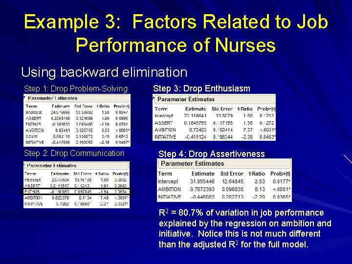
Example 3: Factors Related to Job Performance of Nurses Using backward elimination Step 1: Drop Problem-Solving Step 2: Drop Communication Step 3: Drop Enthusiasm Step 4: Drop Assertiveness R 2 = 80. 7% of variation in job performance explained by the regression on ambition and initiative. Notice this is not much different than the adjusted R 2 for the full model.

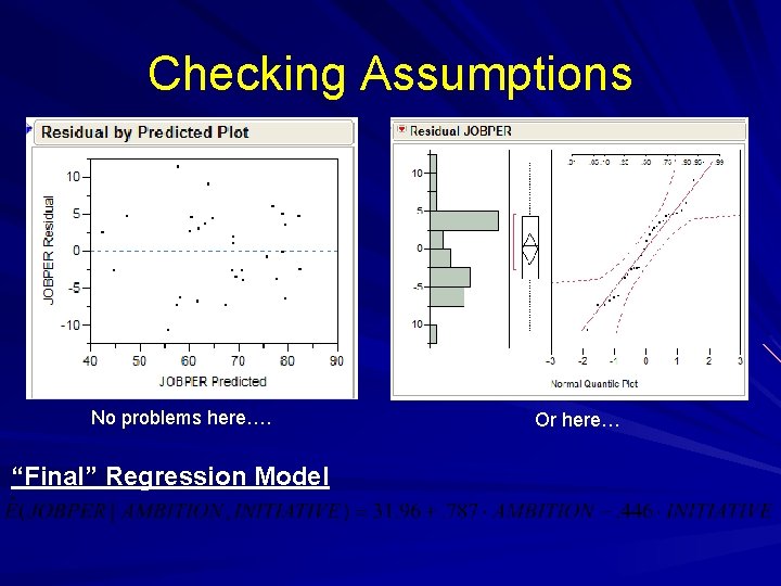
Checking Assumptions No problems here…. “Final” Regression Model Or here…

Summary • Two-sample t-tests, one-way, and two-way ANOVA are all really just regression models with nominal predictors. • Analysis of Covariance (ANCOVA) is also just regression where we are interested in making population/treatment comparisons adjusting for the potential effects of other factors/covariates. • Multiple regression in general is process of estimating the mean response of a variable (Y) using multiple predictors/independent variables, E(Y|X 1, …, Xp).

Summary • Partial correlation and added variable or leverage plots help understand the relationship between the response and an individual independent variable adjusting for the other independent variables being considered. • Assumption checking is basically the same as it was for simple linear regression.

Summary • When problems are evident general remedies include: • Transforming the response (Y) • Transforming the predictors • Adding nonlinear terms to the model like squared terms (Xi 2) or including interaction terms. • Still need to be aware of “strange” observations, i. e. outliers and influential points.