Correlation and Simple Linear Regression Correlation Analysis Correlation

Correlation and Simple Linear Regression

Correlation Analysis Correlation analysis is used to describe the degree to which one variable is linearly related to another. There are two measures for describing correlation: 1. The Coefficient of Correlation 2. The Coefficient of Determination

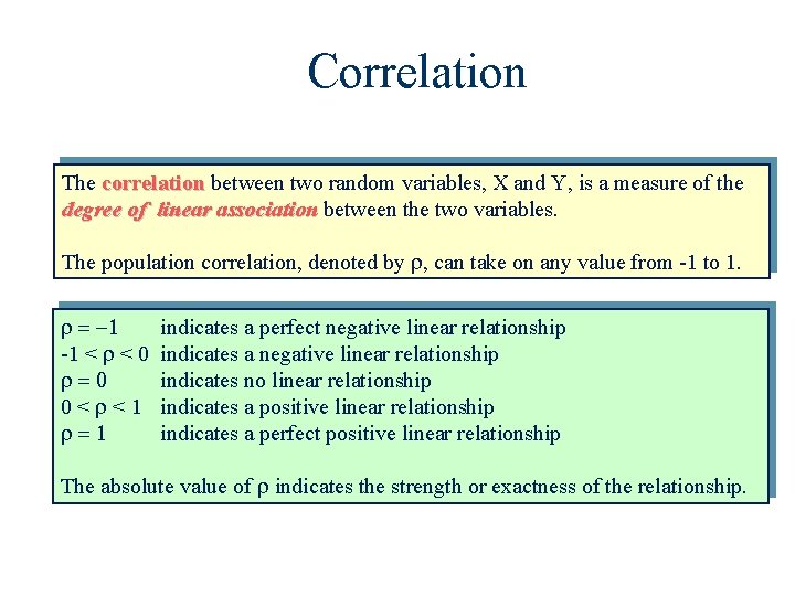
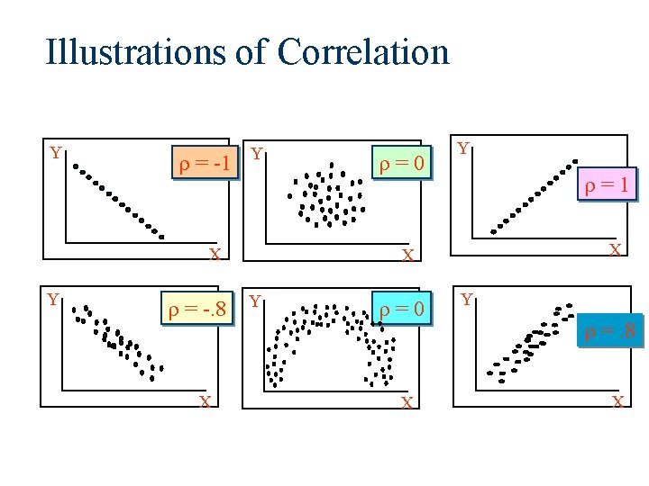
Correlation The correlation between two random variables, X and Y, is a measure of the degree of linear association between the two variables. The population correlation, denoted by , can take on any value from -1 to 1. -1 < < 0 0< <1 indicates a perfect negative linear relationship indicates a negative linear relationship indicates no linear relationship indicates a positive linear relationship indicates a perfect positive linear relationship The absolute value of indicates the strength or exactness of the relationship.

Illustrations of Correlation Y = -1 Y X Y = -. 8 X = 0 Y = 1 X X Y = 0 X Y =. 8 X

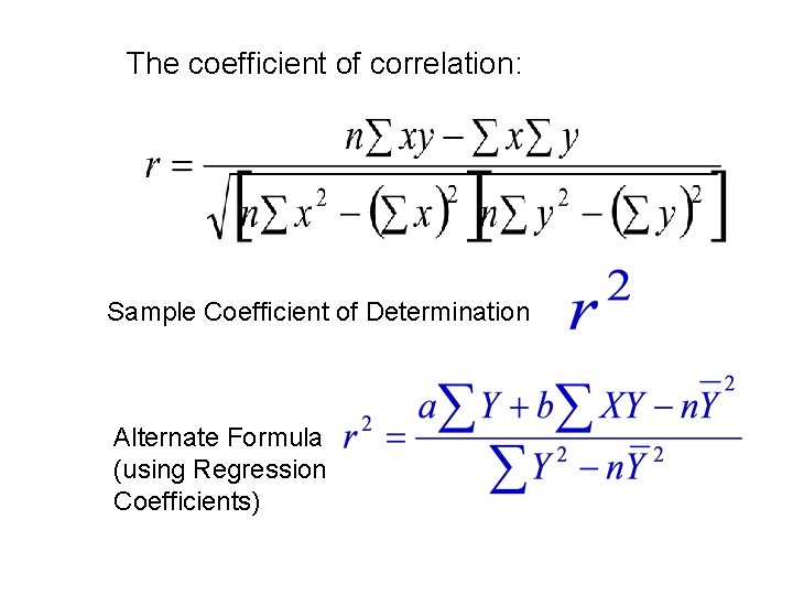
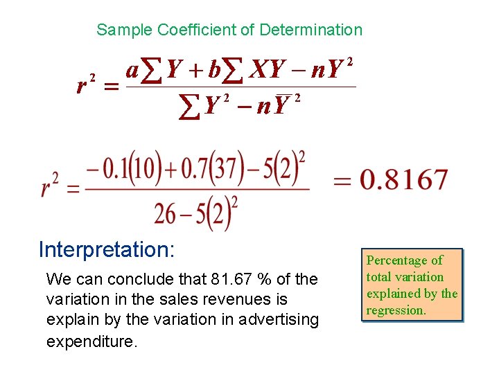
The coefficient of correlation: Sample Coefficient of Determination Alternate Formula (using Regression Coefficients)

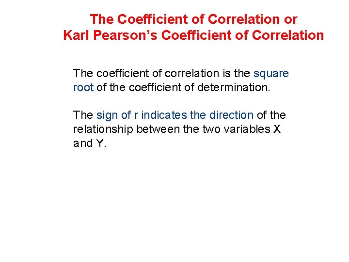
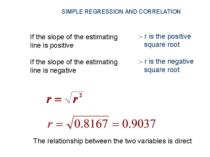
The Coefficient of Correlation or Karl Pearson’s Coefficient of Correlation The coefficient of correlation is the square root of the coefficient of determination. The sign of r indicates the direction of the relationship between the two variables X and Y.

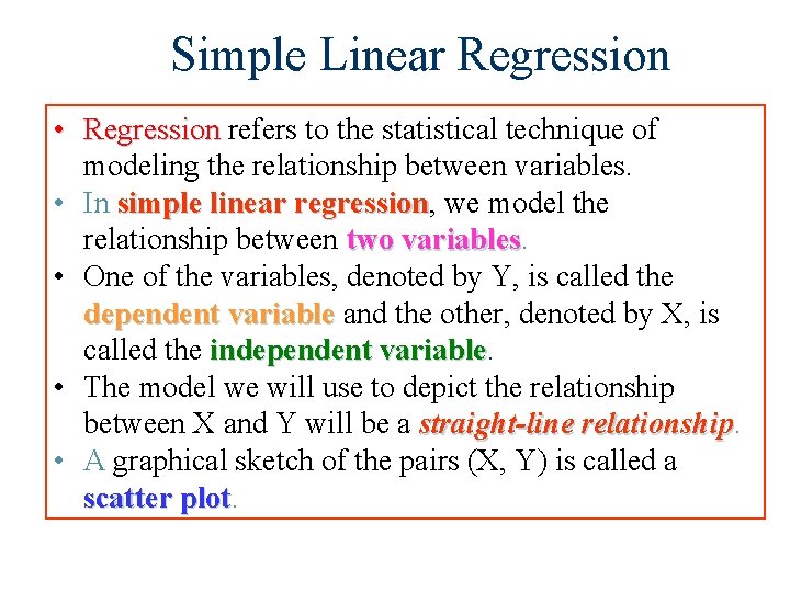
Simple Linear Regression • Regression refers to the statistical technique of modeling the relationship between variables. • In simple linear regression, regression we model the relationship between two variables • One of the variables, denoted by Y, is called the dependent variable and the other, denoted by X, is called the independent variable • The model we will use to depict the relationship between X and Y will be a straight-line relationship • A graphical sketch of the pairs (X, Y) is called a scatter plot

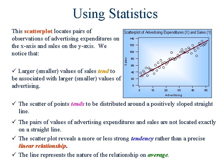
Using Statistics Scatterplot of Advertising Expenditures (X) and Sales (Y) 140 120 100 S ale s This scatterplot locates pairs of observations of advertising expenditures on the x-axis and sales on the y-axis. We notice that: ü Larger (smaller) values of sales tend to be associated with larger (smaller) values of advertising. 80 60 40 20 0 0 10 20 30 40 50 A d ve rtising ü The scatter of points tends to be distributed around a positively sloped straight line. ü The pairs of values of advertising expenditures and sales are not located exactly on a straight line. ü The scatter plot reveals a more or less strong tendency rather than a precise linear relationship. ü The line represents the nature of the relationship on average.

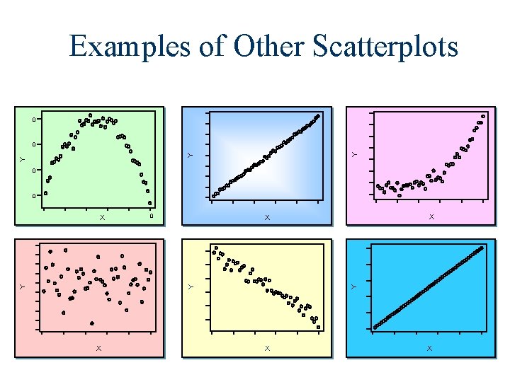
Examples of Other Scatterplots 0 Y Y Y 0 0 X X X Y Y Y X X X

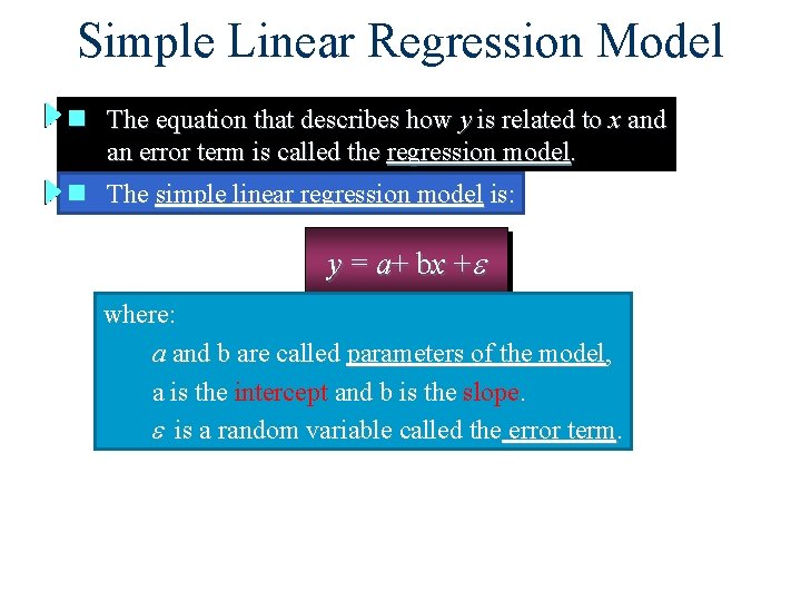
Simple Linear Regression Model n The equation that describes how y is related to x and an error term is called the regression model. n The simple linear regression model is: y = a+ bx +e where: a and b are called parameters of the model, a is the intercept and b is the slope. e is a random variable called the error term.

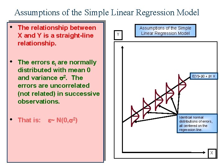
Assumptions of the Simple Linear Regression Model • • • The relationship between X and Y is a straight-line relationship. The errors i are normally distributed with mean 0 and variance 2. The errors are uncorrelated (not related) in successive observations. That is: ~ N(0, 2) Y Assumptions of the Simple Linear Regression Model E[Y]= 0 + 1 X Identical normal distributions of errors, all centered on the regression line. X

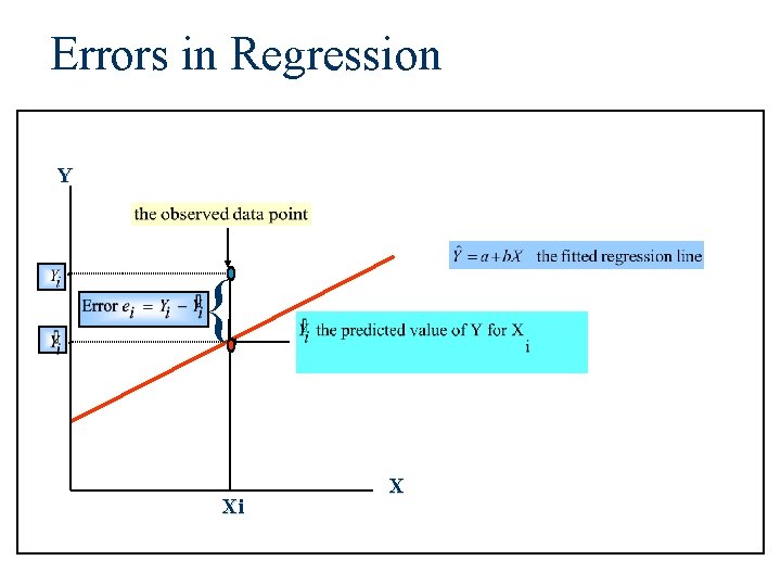
Errors in Regression Y . { Xi X

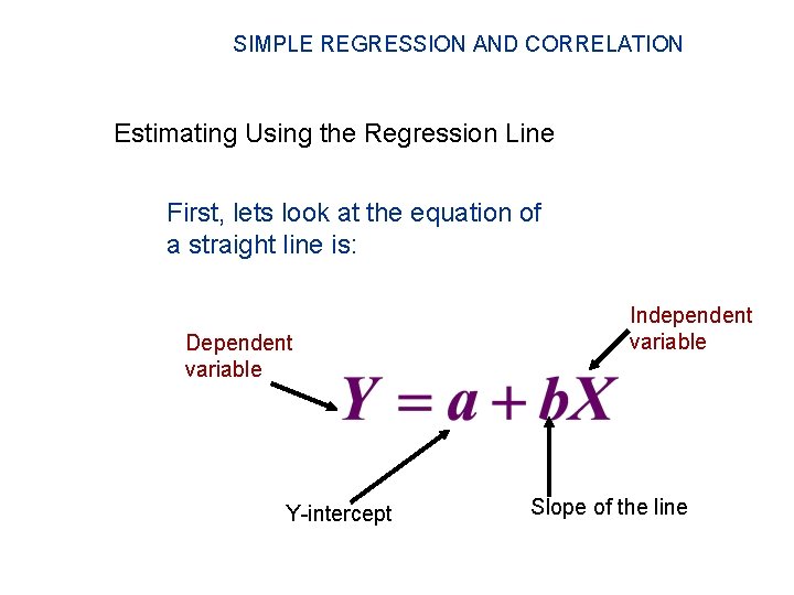
SIMPLE REGRESSION AND CORRELATION Estimating Using the Regression Line First, lets look at the equation of a straight line is: Dependent variable Y-intercept Independent variable Slope of the line

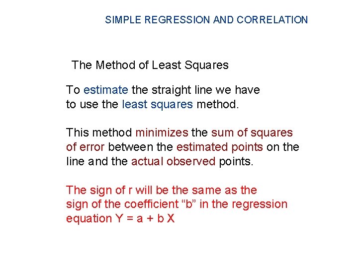
SIMPLE REGRESSION AND CORRELATION The Method of Least Squares To estimate the straight line we have to use the least squares method. This method minimizes the sum of squares of error between the estimated points on the line and the actual observed points. The sign of r will be the same as the sign of the coefficient “b” in the regression equation Y = a + b X

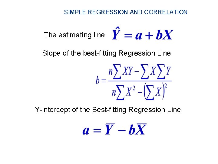
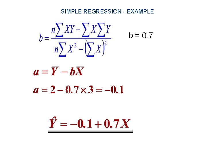
SIMPLE REGRESSION AND CORRELATION The estimating line Slope of the best-fitting Regression Line Y-intercept of the Best-fitting Regression Line

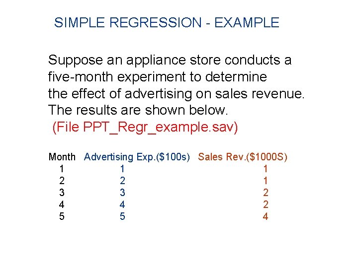
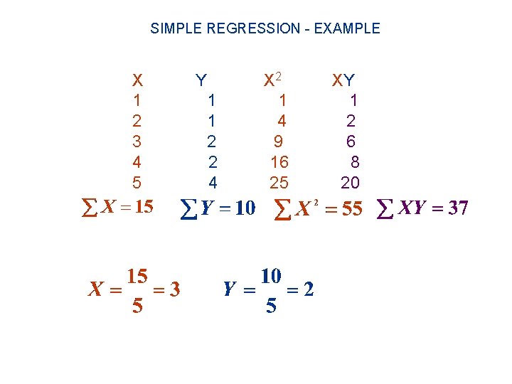
SIMPLE REGRESSION - EXAMPLE Suppose an appliance store conducts a five-month experiment to determine the effect of advertising on sales revenue. The results are shown below. (File PPT_Regr_example. sav) Month Advertising Exp. ($100 s) Sales Rev. ($1000 S) 1 1 1 2 2 1 3 3 2 4 4 2 5 5 4

SIMPLE REGRESSION - EXAMPLE X 1 2 3 4 5 Y 1 1 2 2 4 X 2 1 4 9 16 25 XY 1 2 6 8 20

SIMPLE REGRESSION - EXAMPLE b = 0. 7

Sample Coefficient of Determination Interpretation: We can conclude that 81. 67 % of the variation in the sales revenues is explain by the variation in advertising expenditure. Percentage of total variation explained by the regression.

SIMPLE REGRESSION AND CORRELATION If the slope of the estimating line is positive : - r is the positive square root If the slope of the estimating line is negative : - r is the negative square root The relationship between the two variables is direct

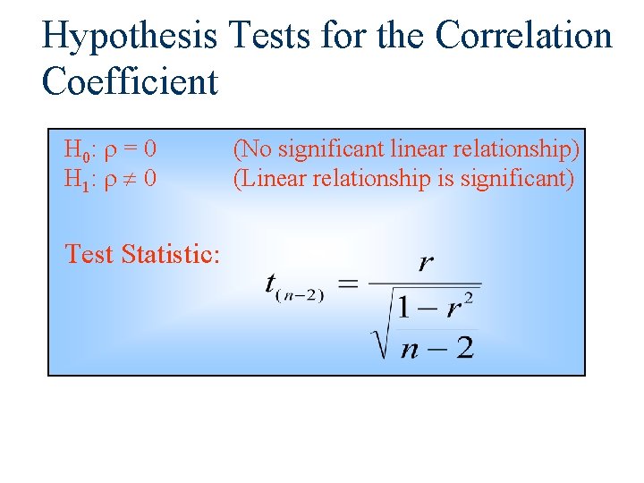
Hypothesis Tests for the Correlation Coefficient H 0: = 0 H 1: 0 Test Statistic: (No significant linear relationship) (Linear relationship is significant)

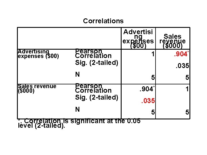
Correlations Advertising expenses ($00) Pearson Correlation Sig. (2 -tailed) Advertisi ng Sales expenses revenue ($00) ($000) 1. 904*. 035 N Sales revenue ($000) Pearson Correlation Sig. (2 -tailed) 5 5 . 904* 1 N *. Correlation is significant at the 0. 05 level (2 -tailed). . 035 5 5

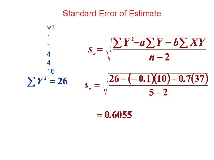
Standard Error of Estimate The standard error of estimate is used to measure the reliability of the estimating equation. It measures the variability or scatter of the observed values around the regression line.

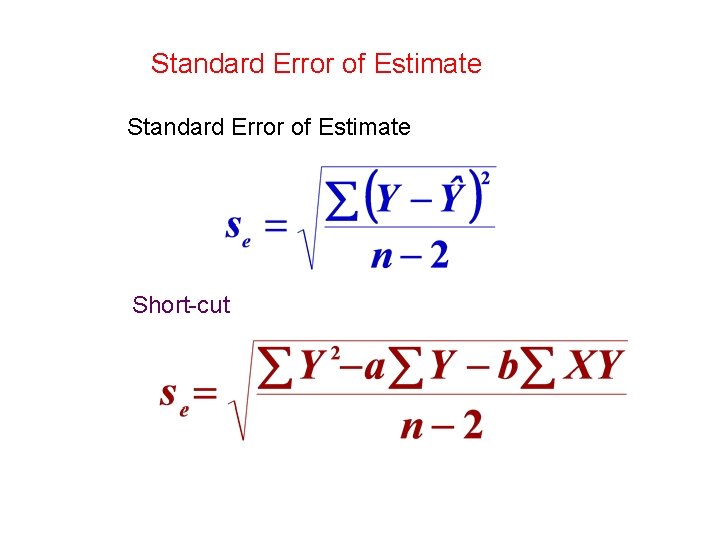
Standard Error of Estimate Short-cut

Standard Error of Estimate Y 2 1 1 4 4 16

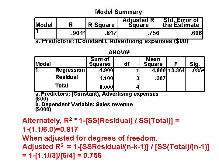
Model Summary Adjusted R Std. Error of Model R R Square the Estimate 1. 904 a. 817. 756. 606 a. Predictors: (Constant), Advertising expenses ($00) ANOVAb Sum of Model Squares df 1 Regression 4. 900 Residual 1. 100 Total 6. 000 Mean Square F Sig. 1 4. 900 13. 364. 035 a 3. 367 4 a. Predictors: (Constant), Advertising expenses ($00) b. Dependent Variable: Sales revenue ($000) Alternately, R 2 = 1 -[SS(Residual) / SS(Total)] = 1 -(1. 1/6. 0)=0. 817 When adjusted for degrees of freedom, Adjusted R 2 = 1 -[SSResidual/(n-k-1)] / [SS(Total)/(n-1)] = 1 -[1. 1//3]/[6/4] = 0. 756

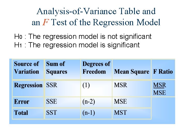
Analysis-of-Variance Table and an F Test of the Regression Model H 0 : The regression model is not significant H 1 : The regression model is significant

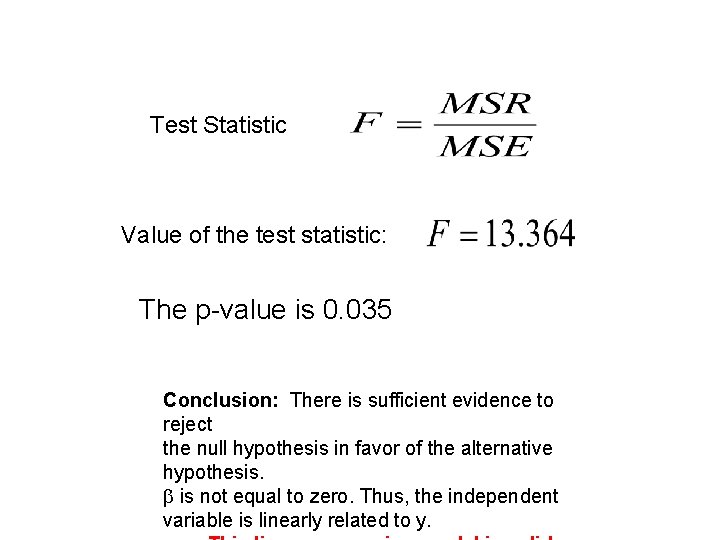
Test Statistic Value of the test statistic: The p-value is 0. 035 Conclusion: There is sufficient evidence to reject the null hypothesis in favor of the alternative hypothesis. is not equal to zero. Thus, the independent variable is linearly related to y.

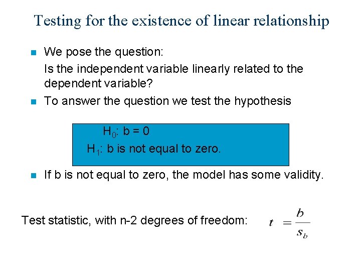
Testing for the existence of linear relationship n n We pose the question: Is the independent variable linearly related to the dependent variable? To answer the question we test the hypothesis H 0: b = 0 H 1: b is not equal to zero. n If b is not equal to zero, the model has some validity. Test statistic, with n-2 degrees of freedom:

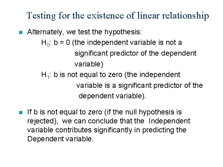
Testing for the existence of linear relationship n Alternately, we test the hypothesis: H 0: b = 0 (the independent variable is not a significant predictor of the dependent variable) H 1: b is not equal to zero (the independent variable is a significant predictor of the dependent variable). n If b is not equal to zero (if the null hypothesis is rejected), we can conclude that the Independent variable contributes significantly in predicting the Dependent variable.

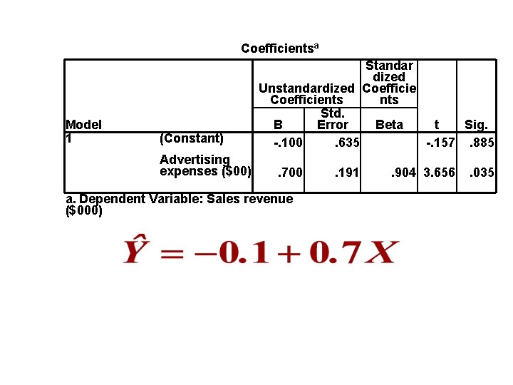
Coefficientsa Model 1 (Constant) Advertising expenses ($00) Standar dized Unstandardized Coefficients Std. B Error Beta t Sig. -. 100. 635 -. 157. 885. 700 a. Dependent Variable: Sales revenue ($000) . 191 . 904 3. 656 . 035

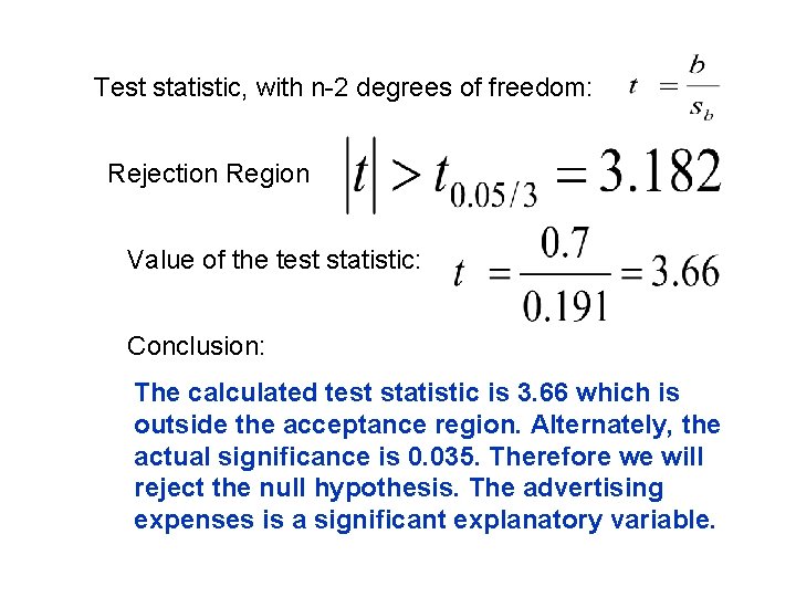
Test statistic, with n-2 degrees of freedom: Rejection Region Value of the test statistic: Conclusion: The calculated test statistic is 3. 66 which is outside the acceptance region. Alternately, the actual significance is 0. 035. Therefore we will reject the null hypothesis. The advertising expenses is a significant explanatory variable.