Linear Regression and Correlation Linear Regression and Correlation

Linear Regression and Correlation

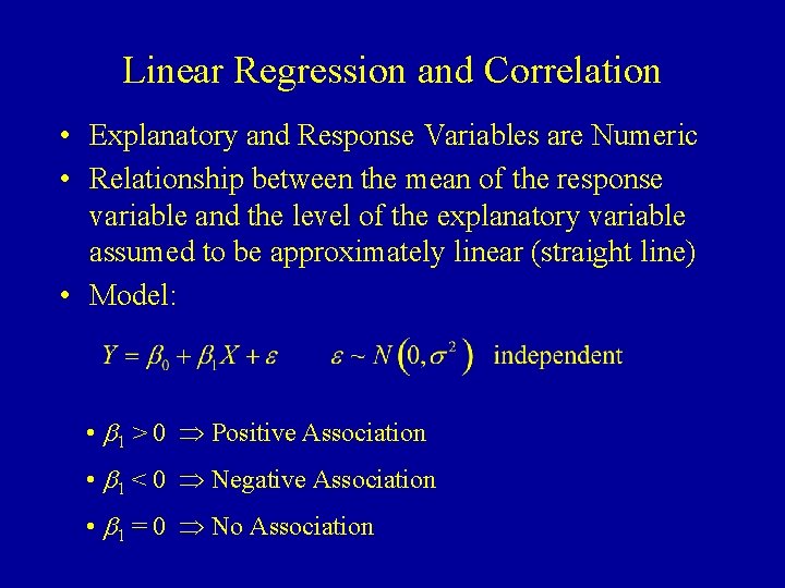
Linear Regression and Correlation • Explanatory and Response Variables are Numeric • Relationship between the mean of the response variable and the level of the explanatory variable assumed to be approximately linear (straight line) • Model: • b 1 > 0 Positive Association • b 1 < 0 Negative Association • b 1 = 0 No Association

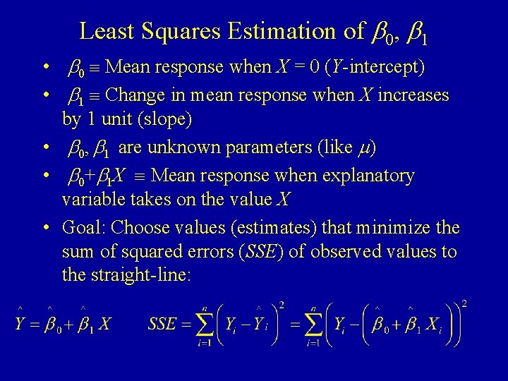
Least Squares Estimation of b 0, b 1 • b 0 Mean response when X = 0 (Y-intercept) • b 1 Change in mean response when X increases by 1 unit (slope) • b 0, b 1 are unknown parameters (like m) • b 0+b 1 X Mean response when explanatory variable takes on the value X • Goal: Choose values (estimates) that minimize the sum of squared errors (SSE) of observed values to the straight-line:

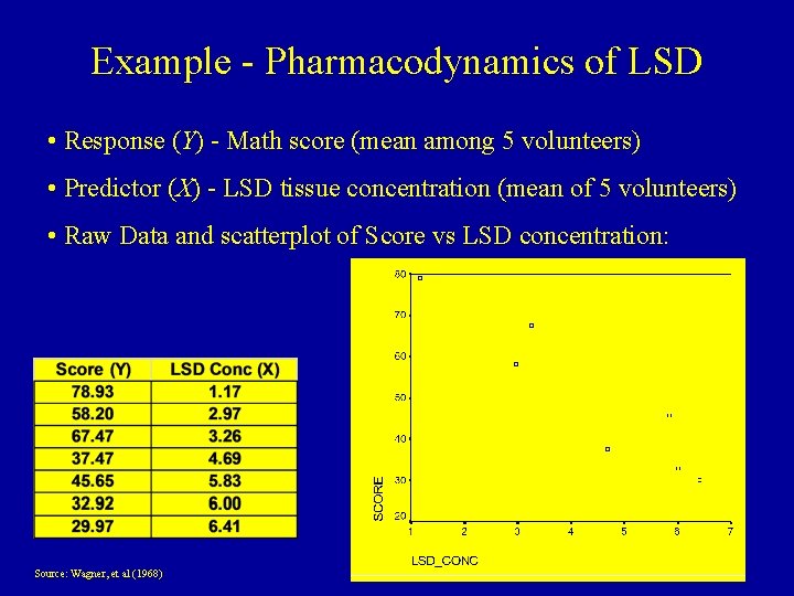
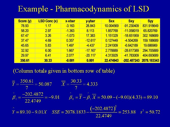
Example - Pharmacodynamics of LSD • Response (Y) - Math score (mean among 5 volunteers) • Predictor (X) - LSD tissue concentration (mean of 5 volunteers) • Raw Data and scatterplot of Score vs LSD concentration: Source: Wagner, et al (1968)

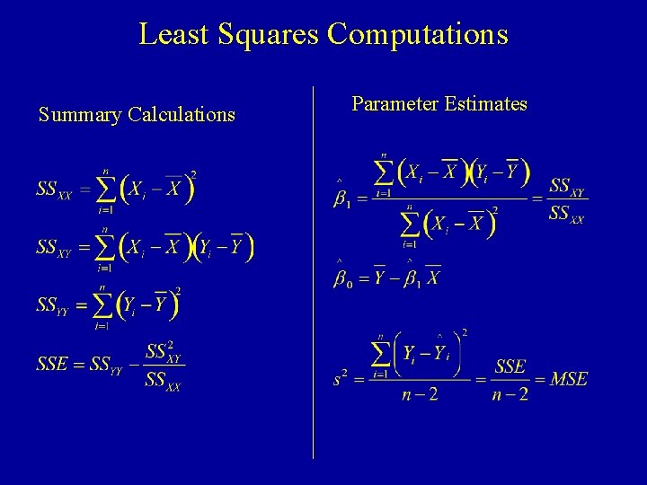
Least Squares Computations Summary Calculations Parameter Estimates

Example - Pharmacodynamics of LSD (Column totals given in bottom row of table)

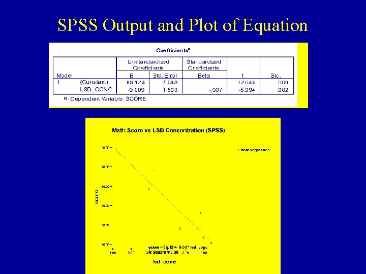
SPSS Output and Plot of Equation

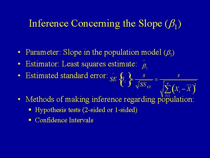
Inference Concerning the Slope (b 1) • Parameter: Slope in the population model (b 1) • Estimator: Least squares estimate: • Estimated standard error: • Methods of making inference regarding population: § Hypothesis tests (2 -sided or 1 -sided) § Confidence Intervals

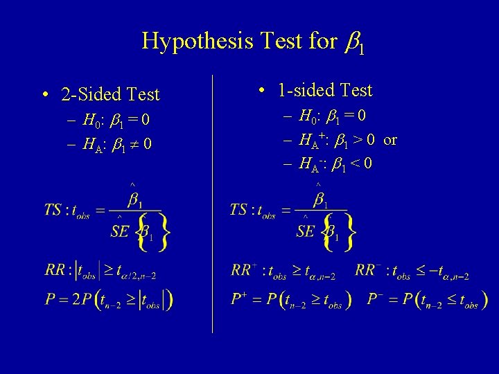
Hypothesis Test for b 1 • 2 -Sided Test – H 0: b 1 = 0 – H A: b 1 0 • 1 -sided Test – H 0: b 1 = 0 – HA+: b 1 > 0 or – H A -: b 1 < 0

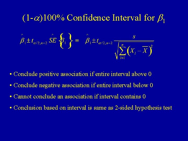
(1 -a)100% Confidence Interval for b 1 • Conclude positive association if entire interval above 0 • Conclude negative association if entire interval below 0 • Cannot conclude an association if interval contains 0 • Conclusion based on interval is same as 2 -sided hypothesis test

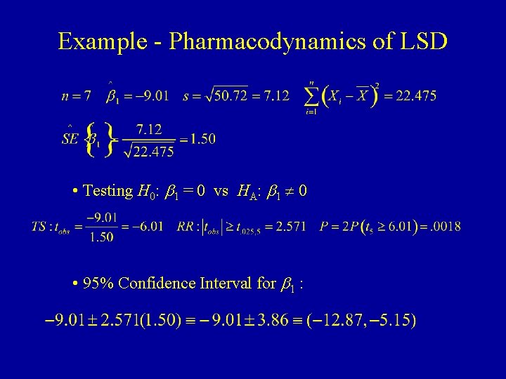
Example - Pharmacodynamics of LSD • Testing H 0: b 1 = 0 vs HA: b 1 0 • 95% Confidence Interval for b 1 :

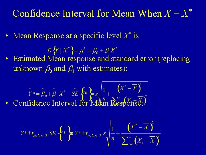
Confidence Interval for Mean When X = X* • Mean Response at a specific level X* is • Estimated Mean response and standard error (replacing unknown b 0 and b 1 with estimates): • Confidence Interval for Mean Response:

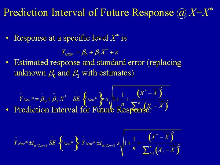
Prediction Interval of Future Response @ X=X* • Response at a specific level X* is • Estimated response and standard error (replacing unknown b 0 and b 1 with estimates): • Prediction Interval for Future Response:

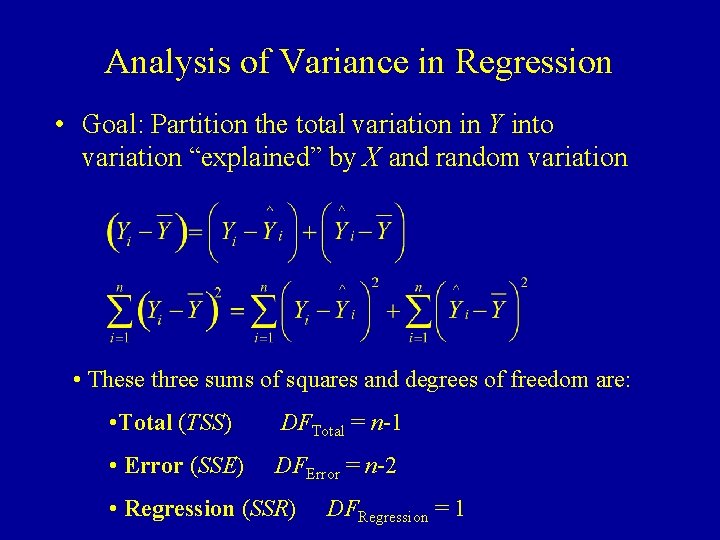
Analysis of Variance in Regression • Goal: Partition the total variation in Y into variation “explained” by X and random variation • These three sums of squares and degrees of freedom are: • Total (TSS) DFTotal = n-1 • Error (SSE) DFError = n-2 • Regression (SSR) DFRegression = 1

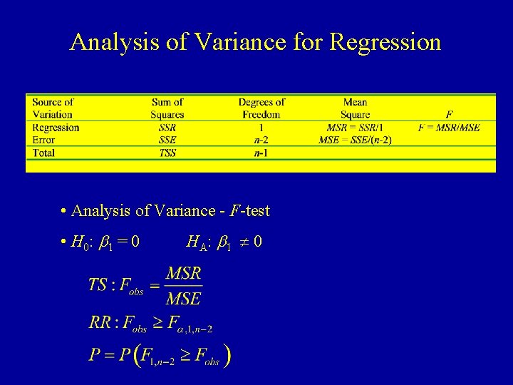
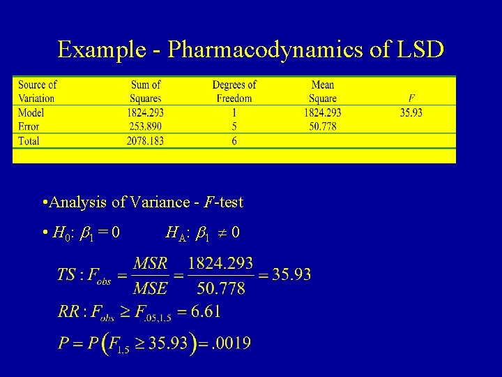
Analysis of Variance for Regression • Analysis of Variance - F-test • H 0: b 1 = 0 HA: b 1 0

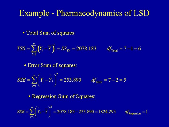
Example - Pharmacodynamics of LSD • Total Sum of squares: • Error Sum of squares: • Regression Sum of Squares:

Example - Pharmacodynamics of LSD • Analysis of Variance - F-test • H 0: b 1 = 0 HA: b 1 0

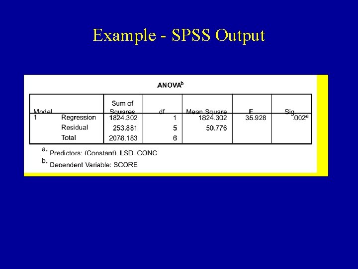
Example - SPSS Output

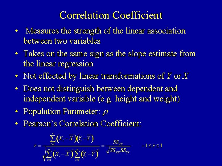
Correlation Coefficient • Measures the strength of the linear association between two variables • Takes on the same sign as the slope estimate from the linear regression • Not effected by linear transformations of Y or X • Does not distinguish between dependent and independent variable (e. g. height and weight) • Population Parameter: r • Pearson’s Correlation Coefficient:

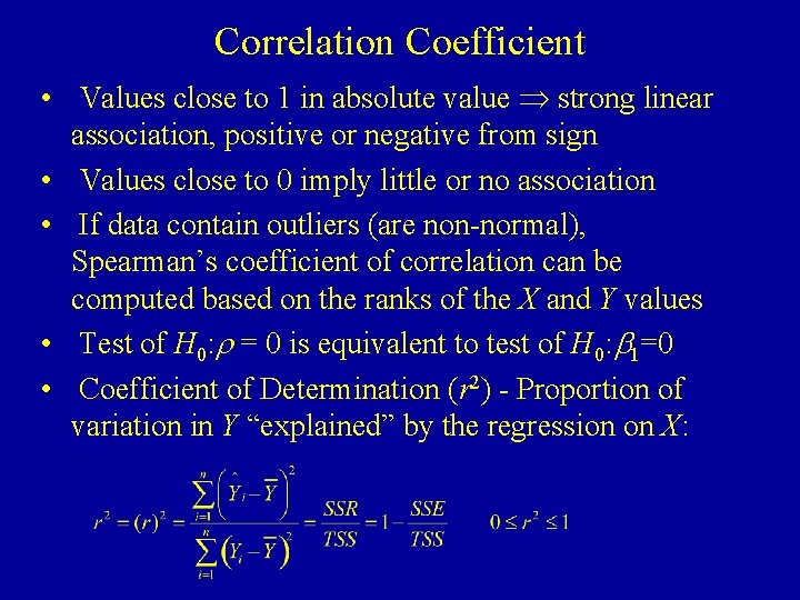
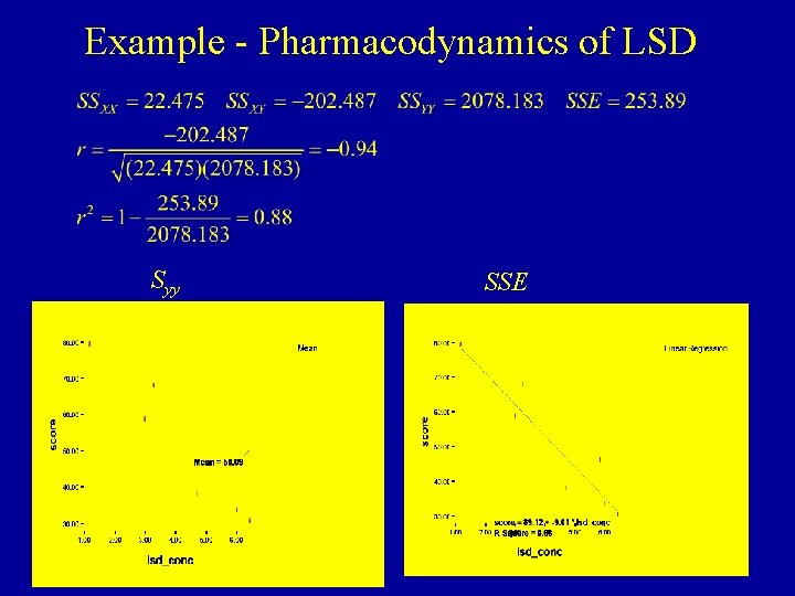
Correlation Coefficient • Values close to 1 in absolute value strong linear association, positive or negative from sign • Values close to 0 imply little or no association • If data contain outliers (are non-normal), Spearman’s coefficient of correlation can be computed based on the ranks of the X and Y values • Test of H 0: r = 0 is equivalent to test of H 0: b 1=0 • Coefficient of Determination (r 2) - Proportion of variation in Y “explained” by the regression on X:

Example - Pharmacodynamics of LSD Syy SSE

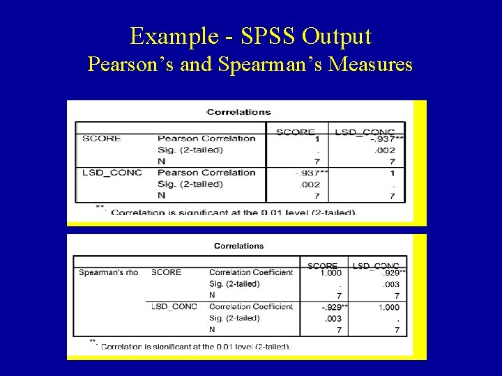
Example - SPSS Output Pearson’s and Spearman’s Measures

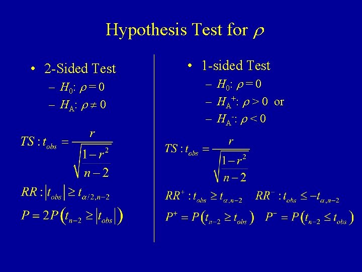
Hypothesis Test for r • 2 -Sided Test – H 0: r = 0 – H A: r 0 • 1 -sided Test – H 0: r = 0 – HA+: r > 0 or – H A -: r < 0

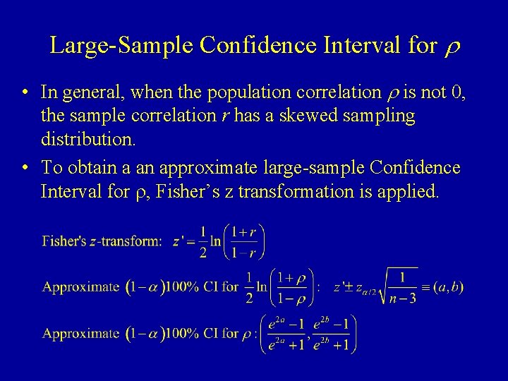
Large-Sample Confidence Interval for r • In general, when the population correlation r is not 0, the sample correlation r has a skewed sampling distribution. • To obtain a an approximate large-sample Confidence Interval for r, Fisher’s z transformation is applied.

Example - Pharmacodynamics of LSD Note that this is hardly a large sample, the Confidence Interval is given to demonstrate calculations

Model Diagnostics • Inferences for the Simple Regression model are based on the following assumptions (which extend to Multiple Regression). • • Relation between Y and X is linear Errors are normally distributed Errors have constant variance Errors are independent • These assumptions can be checked graphically and by formal tests.

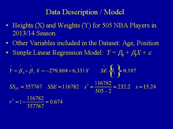
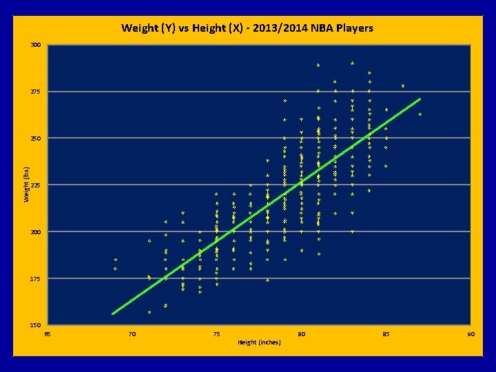
Data Description / Model • Heights (X) and Weights (Y) for 505 NBA Players in 2013/14 Season. • Other Variables included in the Dataset: Age, Position • Simple Linear Regression Model: Y = b 0 + b 1 X + e

Weight (Y) vs Height (X) - 2013/2014 NBA Players 300 275 Weight (lbs) 250 225 200 175 150 65 70 75 Height (inches) 80 85 90

Linearity of Regression (SLR)

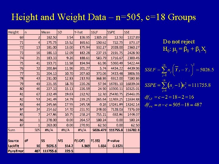
Height and Weight Data – n=505, c=18 Groups Do not reject H 0 : mj = b 0 + b 1 Xj

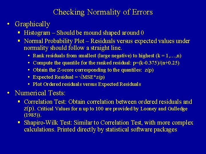
Checking Normality of Errors • Graphically § Histogram – Should be mound shaped around 0 § Normal Probability Plot – Residuals versus expected values under normality should follow a straight line. • • • Rank residuals from smallest (large negative) to highest (k = 1, …, n) Compute the quantile for the ranked residual: p=(k-0. 375)/(n+0. 25) Obtain the Z-score corresponding to the quantiles: z(p) Expected Residual = √MSE*z(p) Plot Ordered residuals versus Expected Residuals • Numerical Tests: § Correlation Test: Obtain correlation between ordered residuals and z(p). Critical Values for n up to 100 are provided by Looney and Gulledge (1985)). § Shapiro-Wilk Test: Similar to Correlation Test, with more complex calculations. Printed directly by statistical software packages

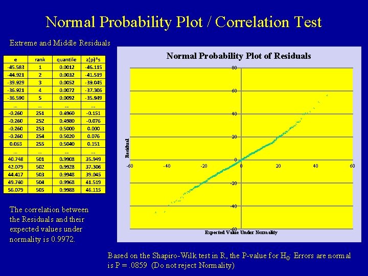
Normal Probability Plot / Correlation Test Extreme and Middle Residuals Normal Probability Plot of Residuals 80 60 40 Residual 20 -60 0 -40 -20 0 20 40 60 -20 The correlation between the Residuals and their expected values under normality is 0. 9972. -40 -60 Expected Value Under Normality Based on the Shapiro-Wilk test in R, the P-value for H 0: Errors are normal is P =. 0859 (Do not reject Normality)

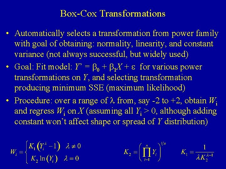
Box-Cox Transformations • Automatically selects a transformation from power family with goal of obtaining: normality, linearity, and constant variance (not always successful, but widely used) • Goal: Fit model: Y’ = b 0 + b 1 X + e for various power transformations on Y, and selecting transformation producing minimum SSE (maximum likelihood) • Procedure: over a range of l from, say -2 to +2, obtain Wi and regress Wi on X (assuming all Yi > 0, although adding constant won’t affect shape or spread of Y distribution)

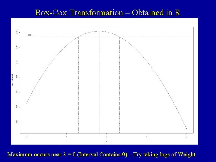
Box-Cox Transformation – Obtained in R Maximum occurs near l = 0 (Interval Contains 0) – Try taking logs of Weight

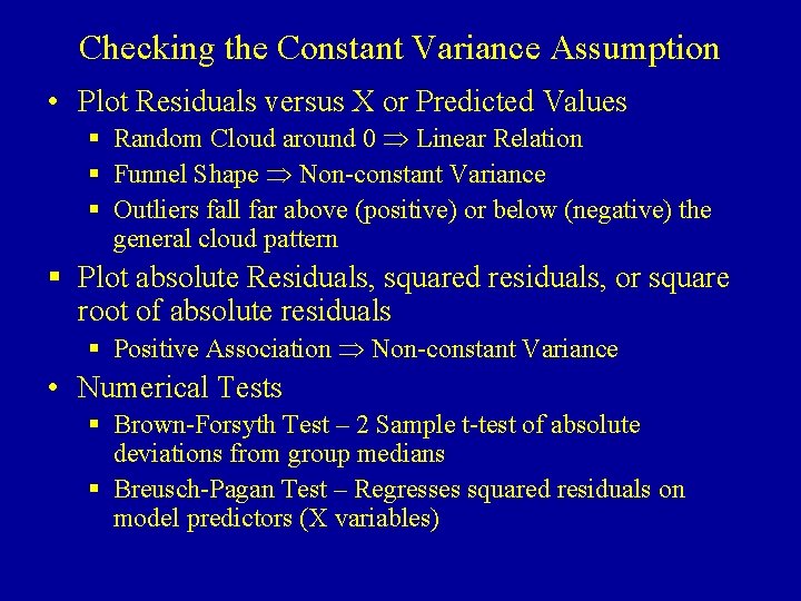
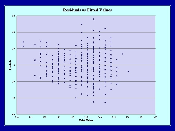
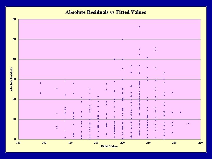
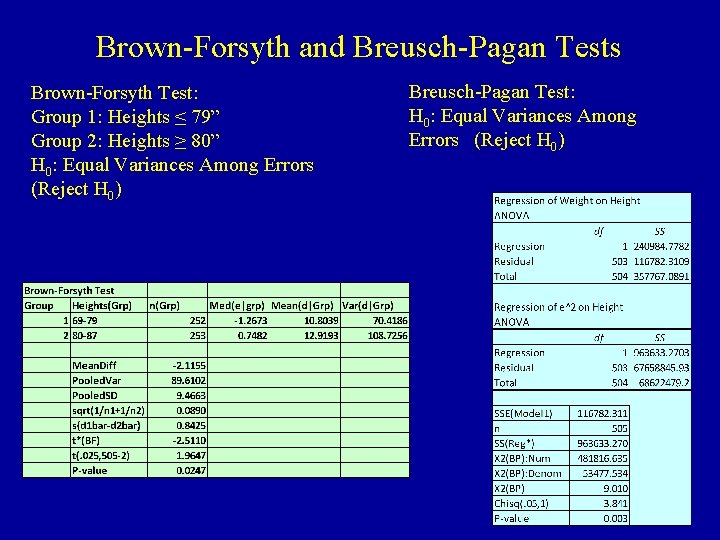
Checking the Constant Variance Assumption • Plot Residuals versus X or Predicted Values § Random Cloud around 0 Linear Relation § Funnel Shape Non-constant Variance § Outliers fall far above (positive) or below (negative) the general cloud pattern § Plot absolute Residuals, squared residuals, or square root of absolute residuals § Positive Association Non-constant Variance • Numerical Tests § Brown-Forsyth Test – 2 Sample t-test of absolute deviations from group medians § Breusch-Pagan Test – Regresses squared residuals on model predictors (X variables)

Residuals vs Fitted Values 60 40 Residuals 20 0 -20 -40 -60 150 165 180 195 210 225 Fitted Values 240 255 270 285 300

Absolute Residuals vs Fitted Values 60 50 Absolute Residuals 40 30 20 10 0 140 160 180 200 220 Fitted Values 240 260 280

Equal (Homogeneous) Variance - I

Equal (Homogeneous) Variance - II

Brown-Forsyth and Breusch-Pagan Tests Brown-Forsyth Test: Group 1: Heights ≤ 79” Group 2: Heights ≥ 80” H 0: Equal Variances Among Errors (Reject H 0) Breusch-Pagan Test: H 0: Equal Variances Among Errors (Reject H 0)

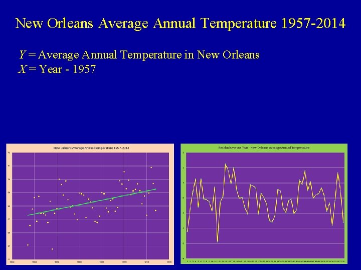
Test For Independence - Durbin-Watson Test

New Orleans Average Annual Temperature 1957 -2014 Y = Average Annual Temperature in New Orleans X = Year - 1957

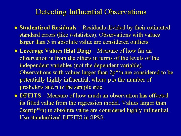
Detecting Influential Observations ¨ Studentized Residuals – Residuals divided by their estimated standard errors (like t-statistics). Observations with values larger than 3 in absolute value are considered outliers. ¨ Leverage Values (Hat Diag) – Measure of how far an observation is from the others in terms of the levels of the independent variables (not the dependent variable). Observations with values larger than 2 p*/n are considered to be potentially highly influential, where p is the number of predictors and n is the sample size. ¨ DFFITS – Measure of how much an observation has effected its fitted value from the regression model. Values larger than 2 sqrt(p*/n) in absolute value are considered highly influential. Use standardized DFFITS in SPSS.

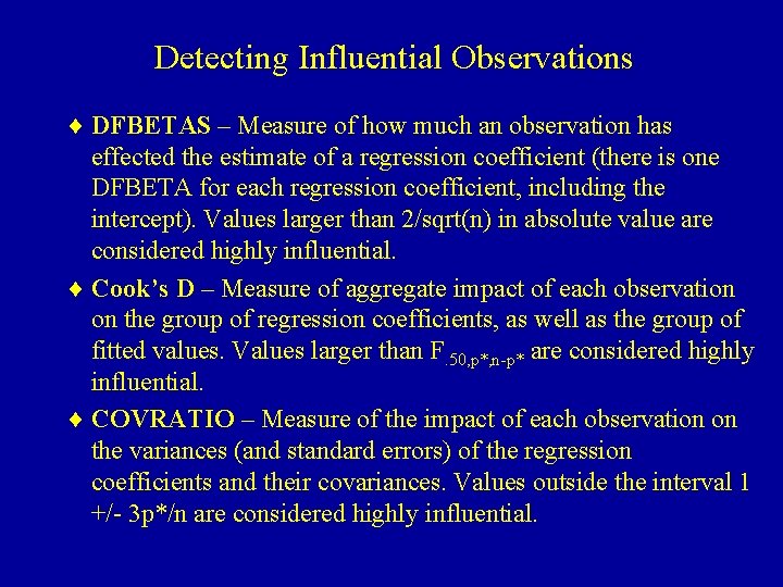
Detecting Influential Observations ¨ DFBETAS – Measure of how much an observation has effected the estimate of a regression coefficient (there is one DFBETA for each regression coefficient, including the intercept). Values larger than 2/sqrt(n) in absolute value are considered highly influential. ¨ Cook’s D – Measure of aggregate impact of each observation on the group of regression coefficients, as well as the group of fitted values. Values larger than F. 50, p*, n-p* are considered highly influential. ¨ COVRATIO – Measure of the impact of each observation on the variances (and standard errors) of the regression coefficients and their covariances. Values outside the interval 1 +/- 3 p*/n are considered highly influential.