Correlation and Regression Analysis Dr Mohammed Alahmed GOALS

Correlation and Regression Analysis Dr. Mohammed Alahmed

GOALS • Understand interpret the terms dependent and independent variable. • Calculate and interpret the coefficient of correlation, the coefficient of determination, and the standard error of estimate. • Conduct a test of hypothesis to determine whether the coefficient of correlation in the population is zero. • Calculate the least squares regression line. • Predict the value of a dependent variable based on the value of at least one independent variable. • Explain the impact of changes in an independent variable on the dependent variable. Dr. Mohammed Alahmed

Introduction • Correlation and regression analysis are related in the sense that both deal with relationships among variables. • For example, we may be interested in studying the relationship between blood pressure and age, height and weight…. • The nature and strength of the relationship between variables may be examined by Correlation and Regression analysis. Dr. Mohammed Alahmed

Correlation Analysis • The term “correlation” refers to a measure of the strength of association between two variables. • Finding the relationship between two quantitative variables without being able to infer causal relationships • Correlation is a statistical technique used to determine the degree to which two variables are related. Dr. Mohammed Alahmed

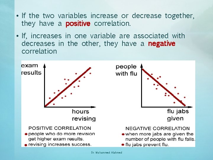
• If the two variables increase or decrease together, they have a positive correlation. • If, increases in one variable are associated with decreases in the other, they have a negative correlation Dr. Mohammed Alahmed

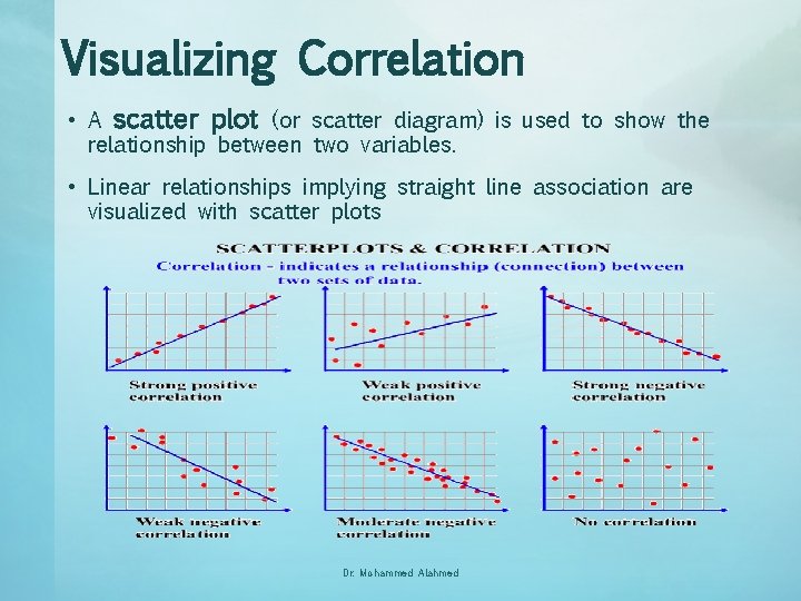
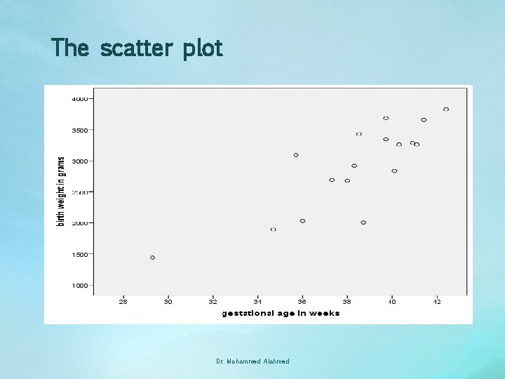
Visualizing Correlation • A scatter plot (or scatter diagram) is used to show the relationship between two variables. • Linear relationships implying straight line association are visualized with scatter plots Dr. Mohammed Alahmed

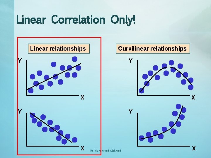
Linear Correlation Only! Linear relationships Curvilinear relationships Y Y X X Y Y X Dr. Mohammed Alahmed X

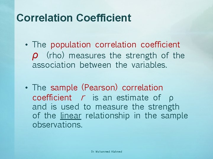
Correlation Coefficient • The population correlation coefficient ρ (rho) measures the strength of the association between the variables. • The sample (Pearson) correlation coefficient r is an estimate of ρ and is used to measure the strength of the linear relationship in the sample observations. Dr. Mohammed Alahmed

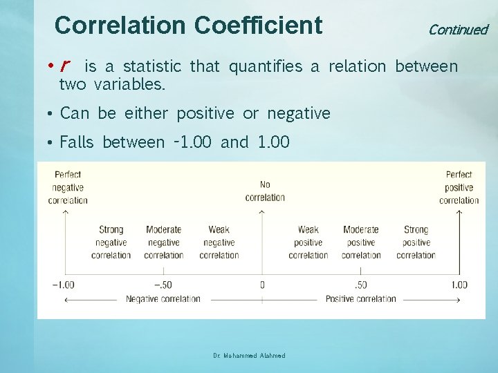
Correlation Coefficient Continued • r is a statistic that quantifies a relation between two variables. • Can be either positive or negative • Falls between -1. 00 and 1. 00 Dr. Mohammed Alahmed

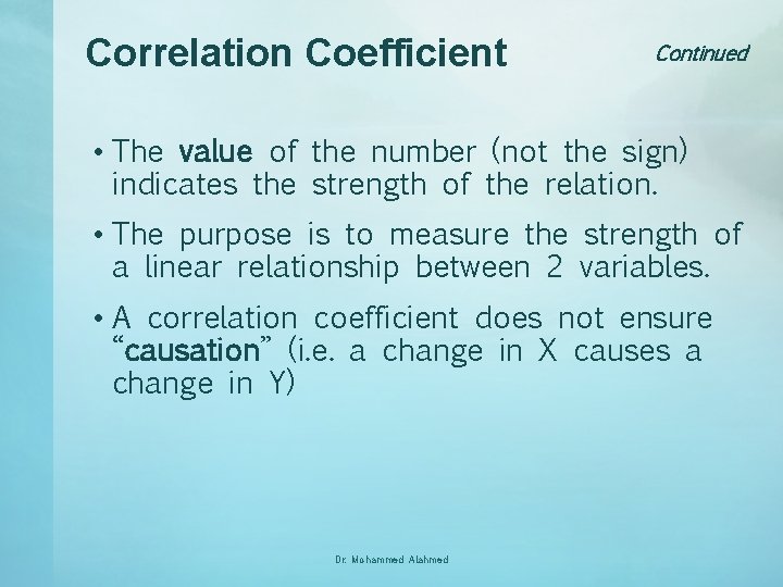
Correlation Coefficient Continued • The value of the number (not the sign) indicates the strength of the relation. • The purpose is to measure the strength of a linear relationship between 2 variables. • A correlation coefficient does not ensure “causation” (i. e. a change in X causes a change in Y) Dr. Mohammed Alahmed

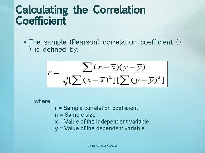
Calculating the Correlation Coefficient • The sample (Pearson) correlation coefficient (r ) is defined by: where: r = Sample correlation coefficient n = Sample size x = Value of the independent variable y = Value of the dependent variable Dr. Mohammed Alahmed

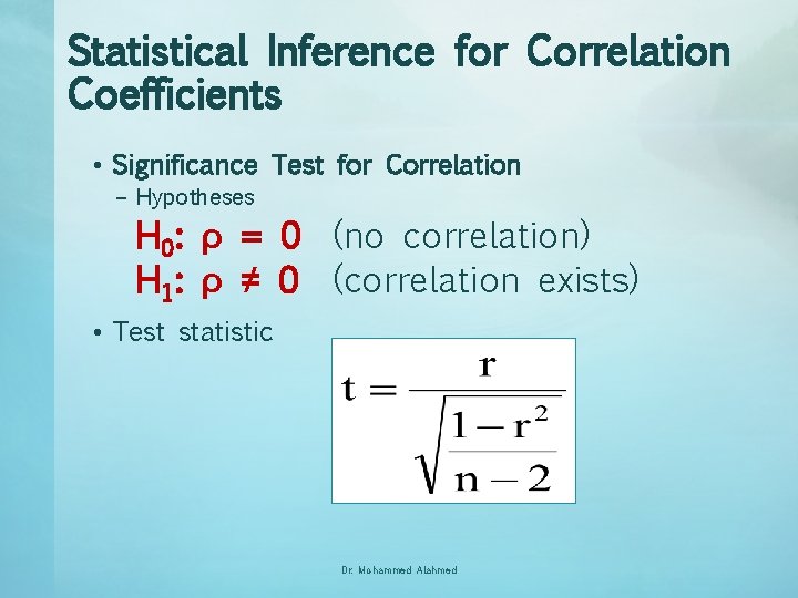
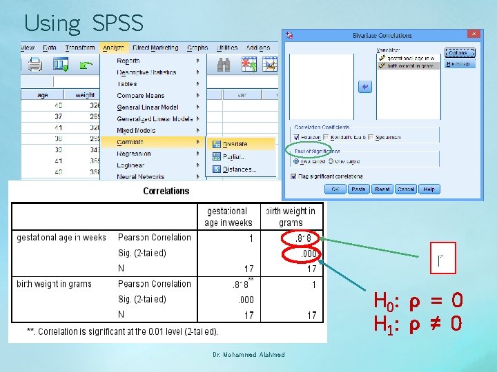
Statistical Inference for Correlation Coefficients • Significance Test for Correlation – Hypotheses H 0: ρ = 0 (no correlation) H 1: ρ ≠ 0 (correlation exists) • Test statistic Dr. Mohammed Alahmed

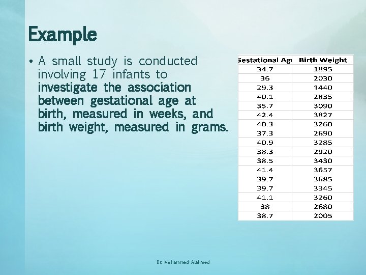
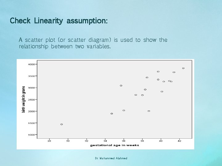
Example • A small study is conducted involving 17 infants to investigate the association between gestational age at birth, measured in weeks, and birth weight, measured in grams. Dr. Mohammed Alahmed

The scatter plot Dr. Mohammed Alahmed

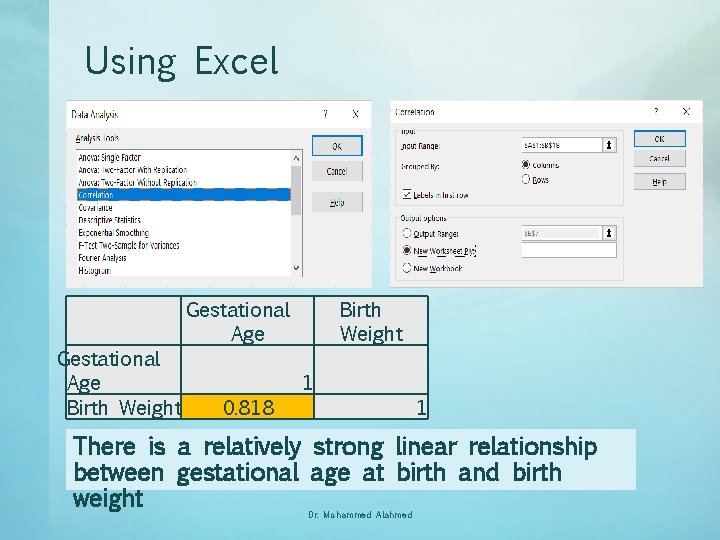
Using Excel Gestational Age Birth Weight Gestational Age 0. 818 Birth Weight 1 1 There is a relatively strong linear relationship between gestational age at birth and birth weight Dr. Mohammed Alahmed

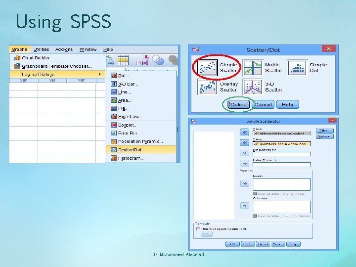
Using SPSS Dr. Mohammed Alahmed

Using SPSS r H 0 : ρ = 0 H 1 : ρ ≠ 0 Dr. Mohammed Alahmed

Cautions about Correlation • Correlation is only a good statistic to use if the relationship is roughly linear. • Correlation can not be used to measure non-linear relationships • Always plot your data to make sure that the relationship is roughly linear! Dr. Mohammed Alahmed

Regression Analysis Regression analysis is used to: – Predict the value of a dependent variable based on the value of at least one independent variable. – Explain the impact of changes in an independent variable on the dependent variable. Dependent variable: the variable we wish to explain. Independent variable: the variable used to explain the dependent variable. Dr. Mohammed Alahmed

Simple Linear Regression Model • Only one independent variable, X • Relationship between X and Y is described by a linear function. • Changes in Y are assumed to be caused by changes in X. Dr. Mohammed Alahmed

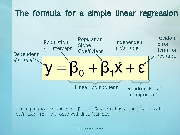
The formula for a simple linear regression Dependent Variable Population y intercept Population Slope Coefficient Independen t Variable Linear component Random Error term, or residual Random Error component The regression coefficients β 0 and β 1 are unknown and have to be estimated from the observed data (sample). Dr. Mohammed Alahmed

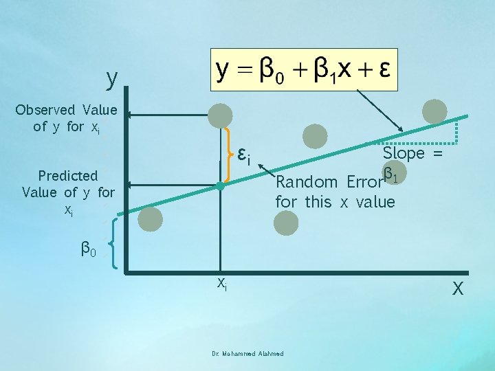
y Observed Value of y for xi εi Predicted Value of y for xi Slope = β 1 Random Error for this x value β 0 xi Dr. Mohammed Alahmed x

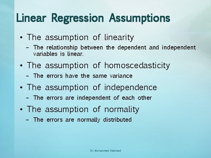
Linear Regression Assumptions • The assumption of linearity – The relationship between the dependent and independent variables is linear. • The assumption of homoscedasticity – The errors have the same variance • The assumption of independence – The errors are independent of each other • The assumption of normality – The errors are normally distributed Dr. Mohammed Alahmed

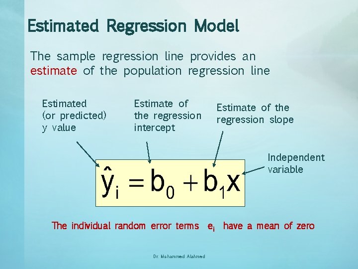
Estimated Regression Model The sample regression line provides an estimate of the population regression line Estimated (or predicted) y value Estimate of the regression intercept Estimate of the regression slope Independent variable The individual random error terms Dr. Mohammed Alahmed ei have a mean of zero

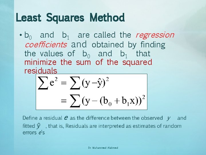
Least Squares Method • b 0 and b 1 are called the regression coefficients and obtained by finding the values of b 0 and b 1 that minimize the sum of the squared residuals Dr. Mohammed Alahmed

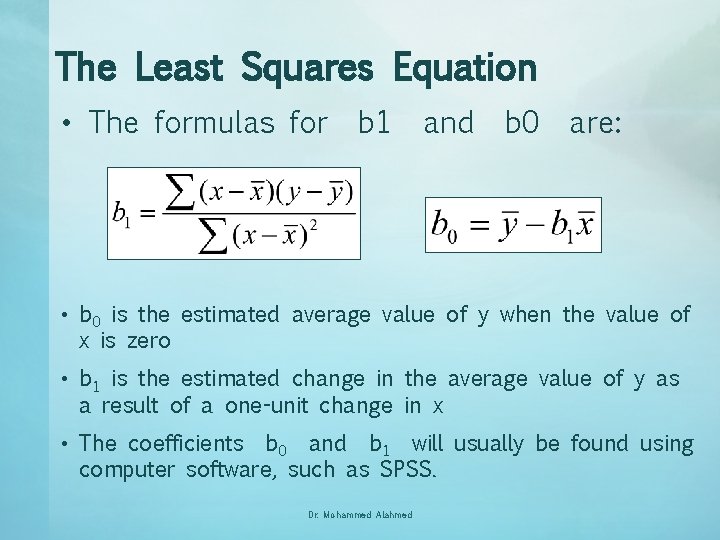
The Least Squares Equation • The formulas for b 1 and b 0 are: • b 0 is the estimated average value of y when the value of x is zero • b 1 is the estimated change in the average value of y as a result of a one-unit change in x • The coefficients b 0 and b 1 will usually be found using computer software, such as SPSS. Dr. Mohammed Alahmed

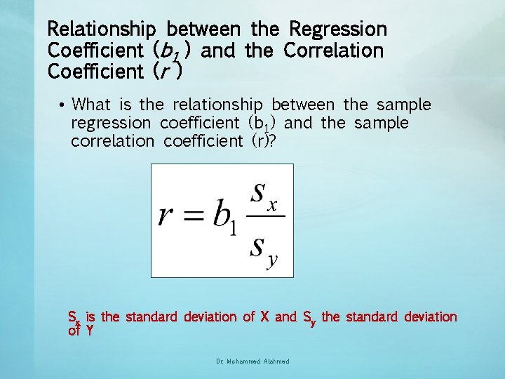
Relationship between the Regression Coefficient (b 1 ) and the Correlation Coefficient (r ) • What is the relationship between the sample regression coefficient (b 1) and the sample correlation coefficient (r)? Sx is the standard deviation of X and Sy the standard deviation of Y Dr. Mohammed Alahmed

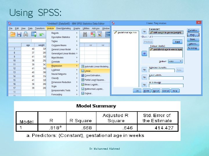
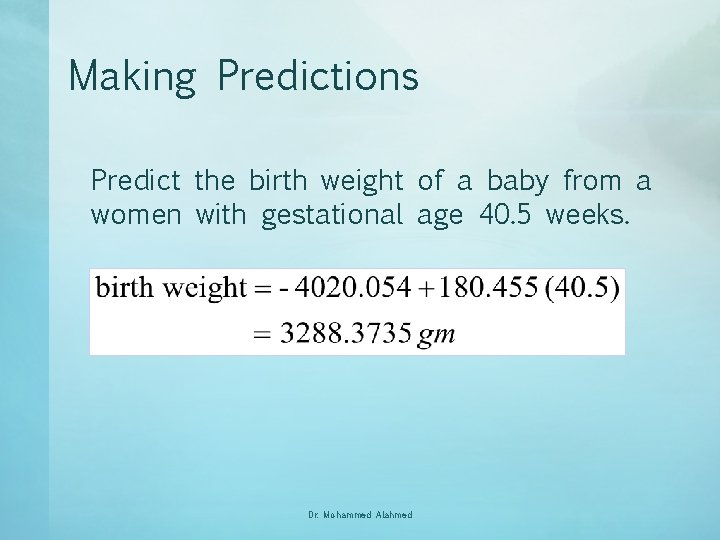
Example • Use the previous example assuming the birth weight is the dependent variable and gestational age as the independent variable. • Fit a linear-regression line relating birth weight to gestational age using these data. • Predict the birth weight of a baby from a women with gestational age 40. 5 weeks. Dr. Mohammed Alahmed

Using SPSS: Dr. Mohammed Alahmed

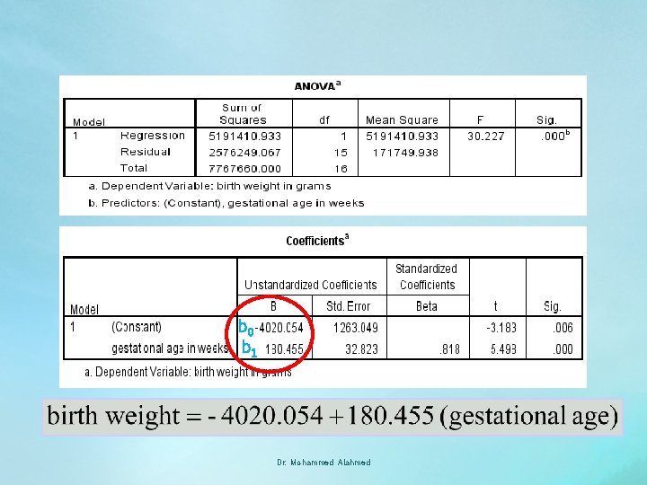
b 0 b 1 Dr. Mohammed Alahmed

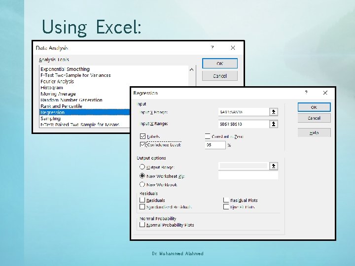
Using Excel: Dr. Mohammed Alahmed

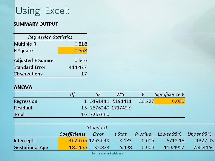
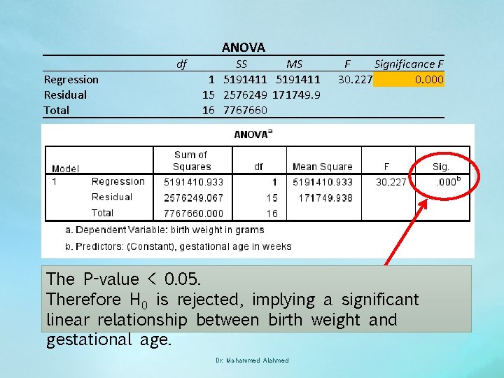
Using Excel: SUMMARY OUTPUT Regression Statistics Multiple R 0. 818 R Square 0. 668 Adjusted R Square Standard Error Observations 0. 646 414. 427 17 ANOVA Regression Residual Total Intercept Gestational Age df SS MS 1 5191411 15 2576249 171749. 9 16 7767660 Standard Coefficients Error - 4020. 05 1263. 049 180. 455 32. 823 F Significance F 30. 227 0. 000 t Stat P-value Lower 95% Upper 95% -3. 183 0. 006 -6712. 18 -1327. 93 5. 498 0. 000 110. 4952 250. 4154 Dr. Mohammed Alahmed

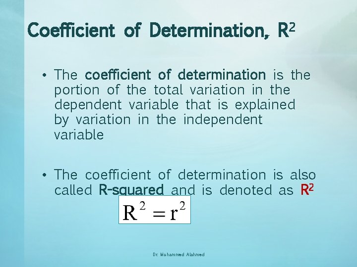
Coefficient of Determination, R 2 • The coefficient of determination is the portion of the total variation in the dependent variable that is explained by variation in the independent variable • The coefficient of determination is also called R-squared and is denoted as R 2 Dr. Mohammed Alahmed

Coefficient of Determination, R 2 • R 2 = Explained variation / Total variation • R 2 is always (%) and between 0% and 100%: • 0% indicates that the model explains none of the variability of the response data around its mean. • 100% indicates that the model explains all the variability of the response data around its mean. • In general, the higher the R-squared, the better the model fits your data. Dr. Mohammed Alahmed

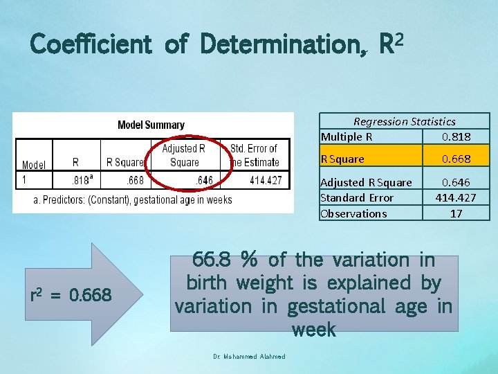
Coefficient of Determination, R 2 Regression Statistics Multiple R 0. 818 R Square Adjusted R Square Standard Error Observations r 2 = 0. 668 0. 646 414. 427 17 66. 8 % of the variation in birth weight is explained by variation in gestational age in week Dr. Mohammed Alahmed

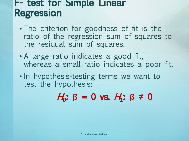
F- test for Simple Linear Regression • The criterion for goodness of fit is the ratio of the regression sum of squares to the residual sum of squares. • A large ratio indicates a good fit, whereas a small ratio indicates a poor fit. • In hypothesis-testing terms we want to test the hypothesis: H 0: β = 0 vs. H 1: β ≠ 0 Dr. Mohammed Alahmed

ANOVA Regression Residual Total df SS MS 1 5191411 15 2576249 171749. 9 16 7767660 F Significance F 30. 227 0. 000 The P-value < 0. 05. Therefore H 0 is rejected, implying a significant linear relationship between birth weight and gestational age. Dr. Mohammed Alahmed

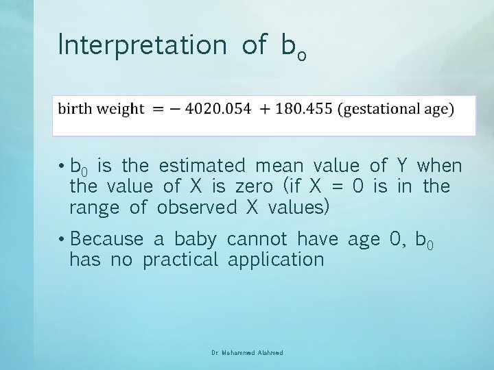
Interpretation of bo • b 0 is the estimated mean value of Y when the value of X is zero (if X = 0 is in the range of observed X values) • Because a baby cannot have age 0, b 0 has no practical application Dr. Mohammed Alahmed

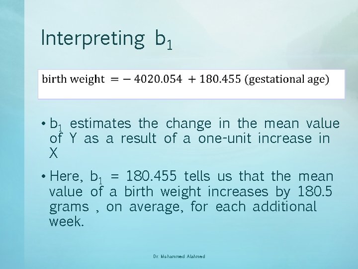
Interpreting b 1 • b 1 estimates the change in the mean value of Y as a result of a one-unit increase in X • Here, b 1 = 180. 455 tells us that the mean value of a birth weight increases by 180. 5 grams , on average, for each additional week. Dr. Mohammed Alahmed

Checking the Regression Assumptions There are two strategies for checking the regression assumptions: 1. Examining the degree to which the variables satisfy the criteria, . e. g. normality and linearity, before the regression is computed by plotting relationships and computing diagnostic statistics. 2. Studying plots of residuals and computing diagnostic statistics after the regression has been computed. Dr. Mohammed Alahmed

Check Linearity assumption: A scatter plot (or scatter diagram) is used to show the relationship between two variables. Dr. Mohammed Alahmed

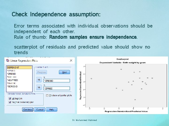
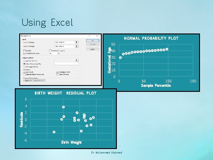
Check Independence assumption: Error terms associated with individual observations should be independent of each other. Rule of thumb: Random samples ensure independence. scatterplot of residuals and predicted value should show no trends Dr. Mohammed Alahmed

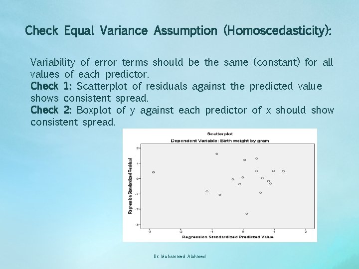
Check Equal Variance Assumption (Homoscedasticity): Variability of error terms should be the same (constant) for all values of each predictor. Check 1: Scatterplot of residuals against the predicted value shows consistent spread. Check 2: Boxplot of y against each predictor of x should show consistent spread. Dr. Mohammed Alahmed

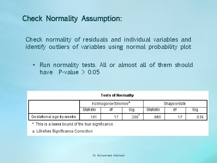
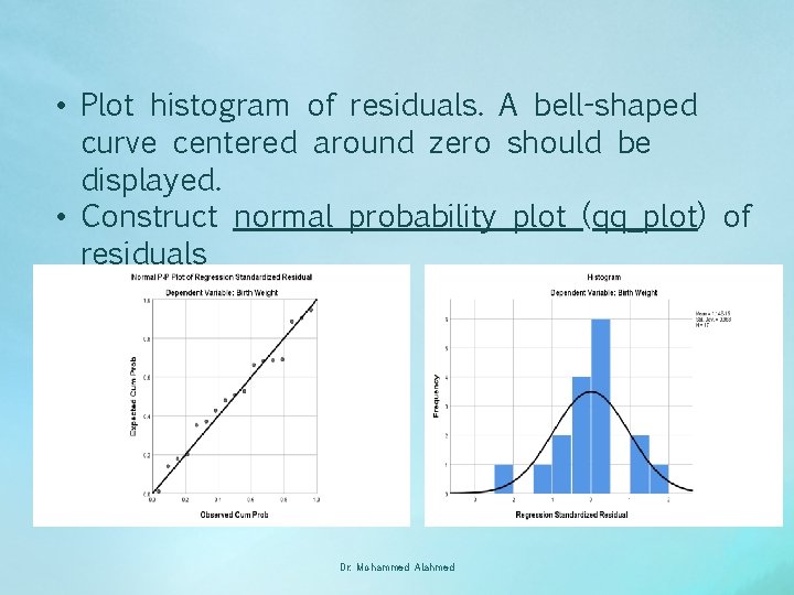
Check Normality Assumption: Check normality of residuals and individual variables and identify outliers of variables using normal probability plot • Run normality tests. All or almost all of them should have P-value > 0. 05 Dr. Mohammed Alahmed

• Plot histogram of residuals. A bell-shaped curve centered around zero should be displayed. • Construct normal probability plot (qq_plot) of residuals Dr. Mohammed Alahmed

Using Excel NORMAL PROBABILITY PLOT Gestational Age 50 40 30 20 10 0 0 BIRTH WEIGHT RESIDUAL PLOT 6 Residuals 4 2 0 -2 -4 -6 Birth Weight Dr. Mohammed Alahmed 50 100 Sample Percentile 150

Making Predictions Predict the birth weight of a baby from a women with gestational age 40. 5 weeks. Dr. Mohammed Alahmed

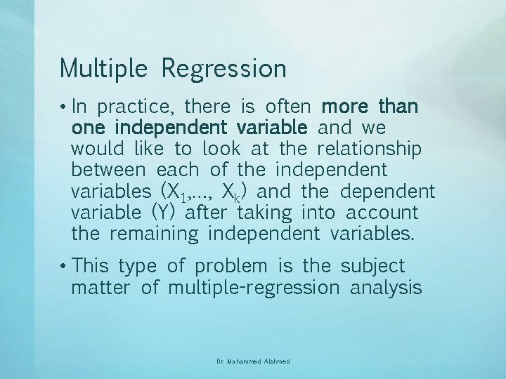
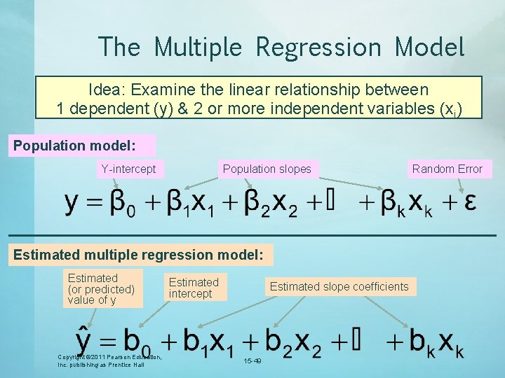
Multiple Regression • In practice, there is often more than one independent variable and we would like to look at the relationship between each of the independent variables (X 1, …, Xk) and the dependent variable (Y) after taking into account the remaining independent variables. • This type of problem is the subject matter of multiple-regression analysis Dr. Mohammed Alahmed

The Multiple Regression Model Idea: Examine the linear relationship between 1 dependent (y) & 2 or more independent variables (xi) Population model: Y-intercept Population slopes Estimated multiple regression model: Estimated (or predicted) value of y Copyright © 2011 Pearson Education, Inc. publishing as Prentice Hall Estimated intercept Estimated slope coefficients 15 -49 Random Error

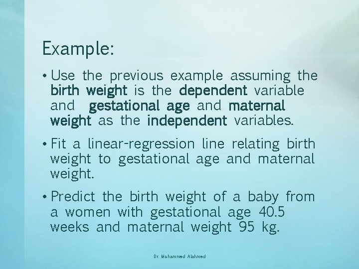
Example: • Use the previous example assuming the birth weight is the dependent variable and gestational age and maternal weight as the independent variables. • Fit a linear-regression line relating birth weight to gestational age and maternal weight. • Predict the birth weight of a baby from a women with gestational age 40. 5 weeks and maternal weight 95 kg. Dr. Mohammed Alahmed

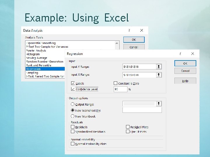
Example: Using Excel Dr. Mohammed Alahmed

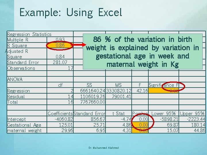
Example: Using Excel Regression Statistics Multiple R R Square Adjusted R Square Standard Error Observations ANOVA Regression Residual Total Intercept Gestational Age maternal weight 0. 93 0. 86 0. 84 281. 07 df 17 2 14 16 86 % of the variation in birth weight is explained by variation in gestational age in week and maternal weight in Kg SS MS 6661640. 24 3330820. 12 1106019. 76 79001. 41 7767660. 00 Coefficients Standard Error -4060. 82 856. 67 125. 01 25. 71 29. 96 6. 95 F Significance F 42. 16 0. 00 t Stat P-value Lower 95% Upper 95% -4. 74 0. 00 -5898. 21 -2223. 44 4. 86 0. 00 69. 87 180. 14 4. 31 0. 00 15. 07 44. 86 Dr. Mohammed Alahmed