Statistical Methods for Particle Physics https indico mitp

Statistical Methods for Particle Physics https: //indico. mitp. uni-mainz. de/event/118/ 11 th International Neutrino Summer School, Schloss Waldthausen, Mainz, 21 May – 1 June, 2018 Glen Cowan Physics Department Royal Holloway, University of London g. cowan@rhul. ac. uk www. pp. rhul. ac. uk/~cowan G. Cowan Neutrino Summer School / Mainz, 25, 26 May 2018 1

Outline Lecture 1: Quick review of probability Parameter estimation, maximum likelihood Statistical tests for discovery and limits Lecture 2: Nuisance parameters and systematic uncertainties Tests from profile likelihood ratio More parameter estimation, Bayesian methods Experimental sensitivity G. Cowan Neutrino Summer School / Mainz, 25, 26 May 2018 2

Some statistics books, papers, etc. G. Cowan, Statistical Data Analysis, Clarendon, Oxford, 1998 R. J. Barlow, Statistics: A Guide to the Use of Statistical Methods in the Physical Sciences, Wiley, 1989 Ilya Narsky and Frank C. Porter, Statistical Analysis Techniques in Particle Physics, Wiley, 2014. L. Lyons, Statistics for Nuclear and Particle Physics, CUP, 1986 F. James. , Statistical and Computational Methods in Experimental Physics, 2 nd ed. , World Scientific, 2006 S. Brandt, Statistical and Computational Methods in Data Analysis, Springer, New York, 1998 (with program library on CD) C. Patrignani et al. (Particle Data Group), Review of Particle Physics, Chin. Phys. C, 40, 100001 (2016); see also pdg. lbl. gov sections on probability, statistics, Monte Carlo G. Cowan Neutrino Summer School / Mainz, 25, 26 May 2018 3

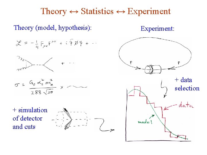
Theory ↔ Statistics ↔ Experiment Theory (model, hypothesis): Experiment: + data selection + simulation of detector and cuts G. Cowan Neutrino Summer School / Mainz, 25, 26 May 2018 4

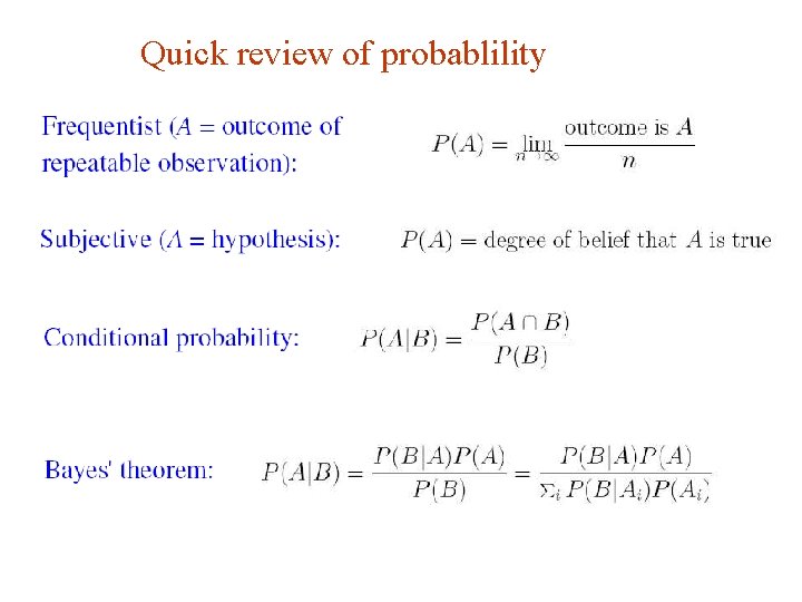
Quick review of probablility G. Cowan Neutrino Summer School / Mainz, 25, 26 May 2018 5

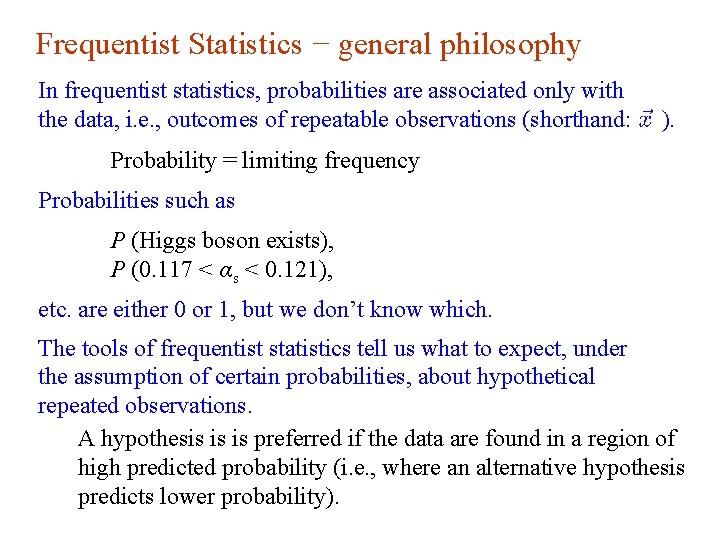
Frequentist Statistics − general philosophy In frequentist statistics, probabilities are associated only with the data, i. e. , outcomes of repeatable observations (shorthand: ). Probability = limiting frequency Probabilities such as P (Higgs boson exists), P (0. 117 < α s < 0. 121), etc. are either 0 or 1, but we don’t know which. The tools of frequentist statistics tell us what to expect, under the assumption of certain probabilities, about hypothetical repeated observations. A hypothesis is is preferred if the data are found in a region of high predicted probability (i. e. , where an alternative hypothesis predicts lower probability). G. Cowan Neutrino Summer School / Mainz, 25, 26 May 2018 6

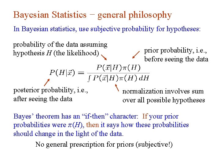
Bayesian Statistics − general philosophy In Bayesian statistics, use subjective probability for hypotheses: probability of the data assuming hypothesis H (the likelihood) posterior probability, i. e. , after seeing the data prior probability, i. e. , before seeing the data normalization involves sum over all possible hypotheses Bayes’ theorem has an “if-then” character: If your prior probabilities were π (H), then it says how these probabilities should change in the light of the data. No general prescription for priors (subjective!) G. Cowan Neutrino Summer School / Mainz, 25, 26 May 2018 7

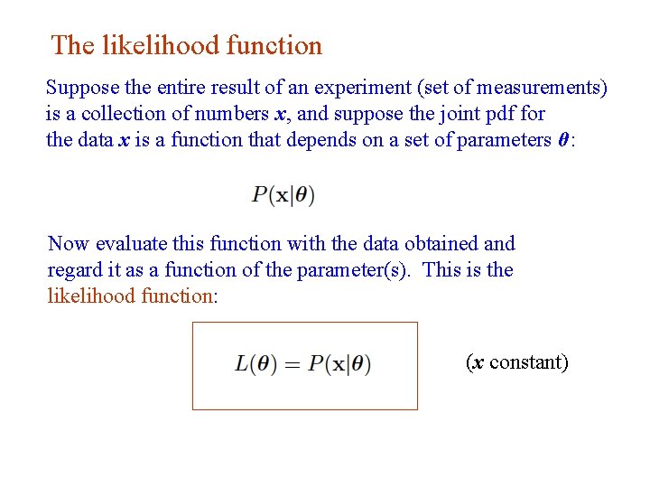
The likelihood function Suppose the entire result of an experiment (set of measurements) is a collection of numbers x, and suppose the joint pdf for the data x is a function that depends on a set of parameters θ: Now evaluate this function with the data obtained and regard it as a function of the parameter(s). This is the likelihood function: (x constant) G. Cowan Neutrino Summer School / Mainz, 25, 26 May 2018 8

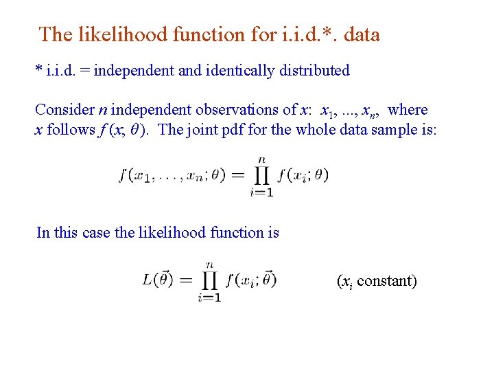
The likelihood function for i. i. d. *. data * i. i. d. = independent and identically distributed Consider n independent observations of x: x 1, . . . , xn, where x follows f (x; θ ). The joint pdf for the whole data sample is: In this case the likelihood function is (xi constant) G. Cowan Neutrino Summer School / Mainz, 25, 26 May 2018 9

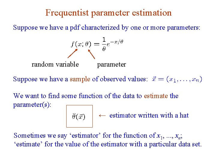
Frequentist parameter estimation Suppose we have a pdf characterized by one or more parameters: random variable parameter Suppose we have a sample of observed values: We want to find some function of the data to estimate the parameter(s): ← estimator written with a hat Sometimes we say ‘estimator’ for the function of x 1, . . . , xn; ‘estimate’ for the value of the estimator with a particular data set. G. Cowan Neutrino Summer School / Mainz, 25, 26 May 2018 10

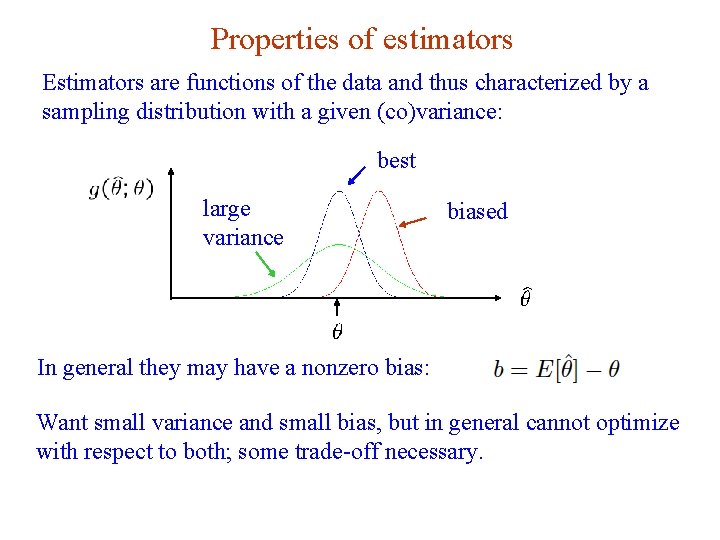
Properties of estimators Estimators are functions of the data and thus characterized by a sampling distribution with a given (co)variance: best large variance biased In general they may have a nonzero bias: Want small variance and small bias, but in general cannot optimize with respect to both; some trade-off necessary. G. Cowan Neutrino Summer School / Mainz, 25, 26 May 2018 11

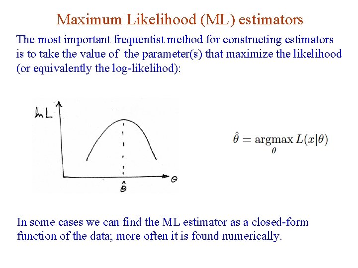
Maximum Likelihood (ML) estimators The most important frequentist method for constructing estimators is to take the value of the parameter(s) that maximize the likelihood (or equivalently the log-likelihod): In some cases we can find the ML estimator as a closed-form function of the data; more often it is found numerically. G. Cowan Neutrino Summer School / Mainz, 25, 26 May 2018 12

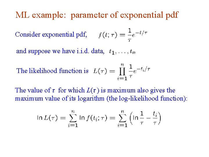
ML example: parameter of exponential pdf Consider exponential pdf, and suppose we have i. i. d. data, The likelihood function is The value of τ for which L(τ ) is maximum also gives the maximum value of its logarithm (the log-likelihood function): G. Cowan Neutrino Summer School / Mainz, 25, 26 May 2018 13

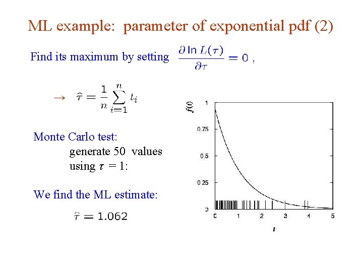
ML example: parameter of exponential pdf (2) Find its maximum by setting → Monte Carlo test: generate 50 values using τ = 1: We find the ML estimate: G. Cowan Neutrino Summer School / Mainz, 25, 26 May 2018 14

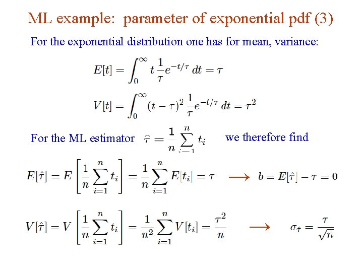
ML example: parameter of exponential pdf (3) For the exponential distribution one has for mean, variance: For the ML estimator we therefore find → → G. Cowan Neutrino Summer School / Mainz, 25, 26 May 2018 15

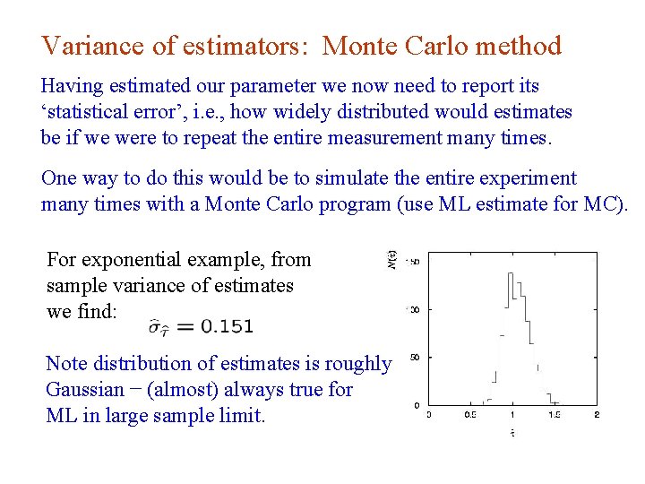
Variance of estimators: Monte Carlo method Having estimated our parameter we now need to report its ‘statistical error’, i. e. , how widely distributed would estimates be if we were to repeat the entire measurement many times. One way to do this would be to simulate the entire experiment many times with a Monte Carlo program (use ML estimate for MC). For exponential example, from sample variance of estimates we find: Note distribution of estimates is roughly Gaussian − (almost) always true for ML in large sample limit. G. Cowan Neutrino Summer School / Mainz, 25, 26 May 2018 16

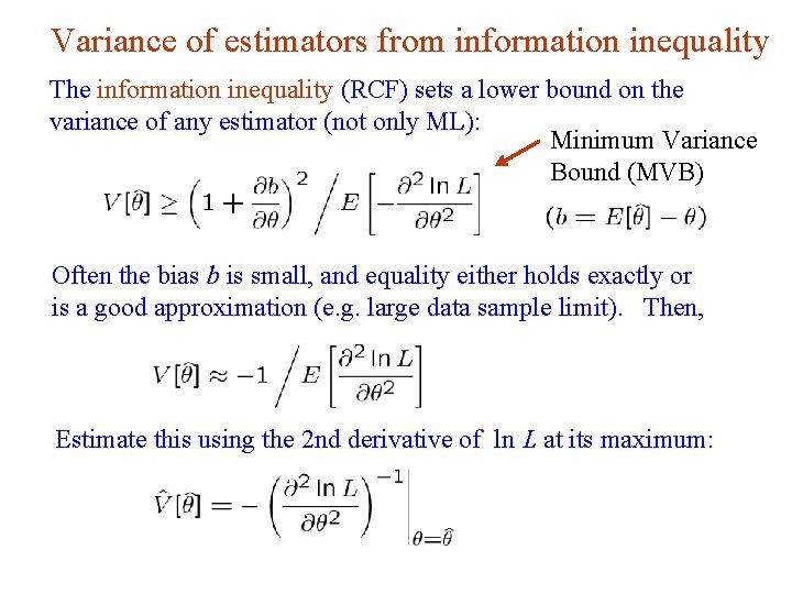
Variance of estimators from information inequality The information inequality (RCF) sets a lower bound on the variance of any estimator (not only ML): Minimum Variance Bound (MVB) Often the bias b is small, and equality either holds exactly or is a good approximation (e. g. large data sample limit). Then, Estimate this using the 2 nd derivative of ln L at its maximum: G. Cowan Neutrino Summer School / Mainz, 25, 26 May 2018 17

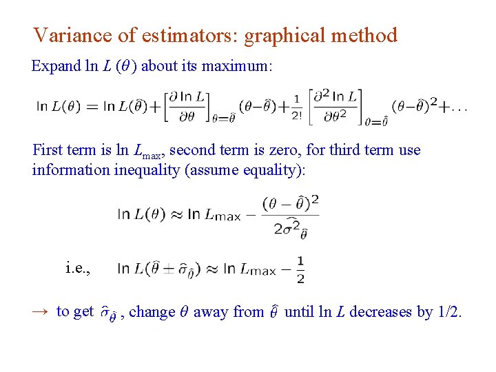
Variance of estimators: graphical method Expand ln L (θ ) about its maximum: First term is ln Lmax, second term is zero, for third term use information inequality (assume equality): i. e. , → to get G. Cowan , change θ away from until ln L decreases by 1/2. Neutrino Summer School / Mainz, 25, 26 May 2018 18

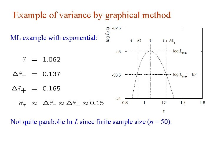
Example of variance by graphical method ML example with exponential: Not quite parabolic ln L since finite sample size (n = 50). G. Cowan Neutrino Summer School / Mainz, 25, 26 May 2018 19

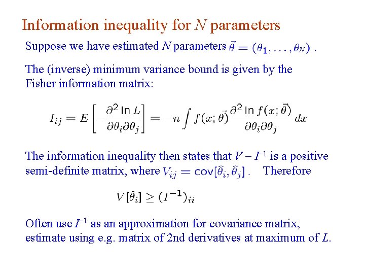
Information inequality for N parameters Suppose we have estimated N parameters N The (inverse) minimum variance bound is given by the Fisher information matrix: The information inequality then states that V - I-1 is a positive semi-definite matrix, where Therefore Often use I-1 as an approximation for covariance matrix, estimate using e. g. matrix of 2 nd derivatives at maximum of L. G. Cowan Neutrino Summer School / Mainz, 25, 26 May 2018 20

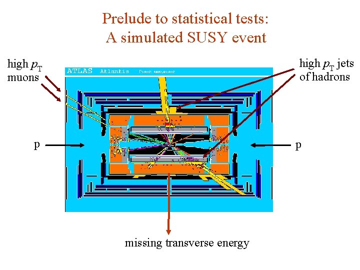
Prelude to statistical tests: A simulated SUSY event high p. T jets of hadrons high p. T muons p p missing transverse energy G. Cowan Neutrino Summer School / Mainz, 25, 26 May 2018 21

Background events This event from Standard Model ttbar production also has high p. T jets and muons, and some missing transverse energy. → can easily mimic a SUSY event. G. Cowan Neutrino Summer School / Mainz, 25, 26 May 2018 22

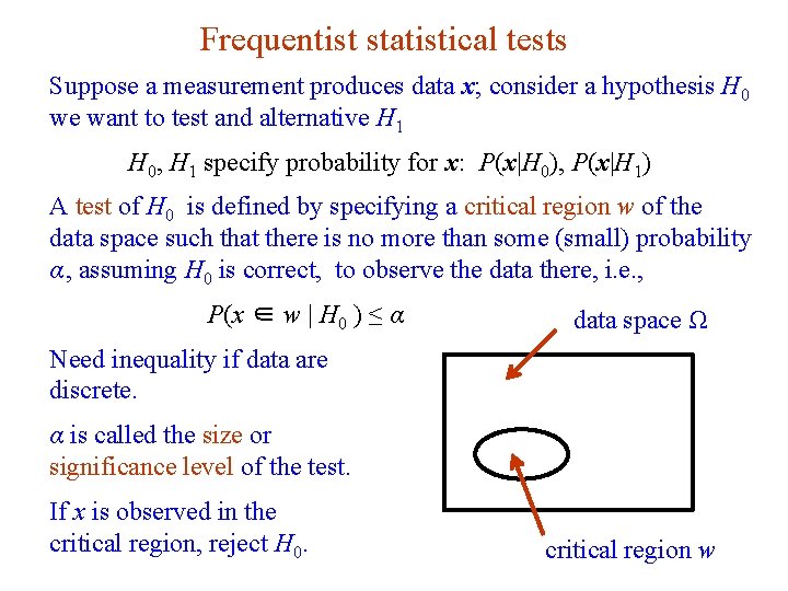
Frequentist statistical tests Suppose a measurement produces data x; consider a hypothesis H 0 we want to test and alternative H 1 H 0, H 1 specify probability for x: P(x|H 0), P(x|H 1) A test of H 0 is defined by specifying a critical region w of the data space such that there is no more than some (small) probability α, assuming H 0 is correct, to observe the data there, i. e. , P(x ∈ w | H 0 ) ≤ α data space Ω Need inequality if data are discrete. α is called the size or significance level of the test. If x is observed in the critical region, reject H 0. G. Cowan critical region w Neutrino Summer School / Mainz, 25, 26 May 2018 23

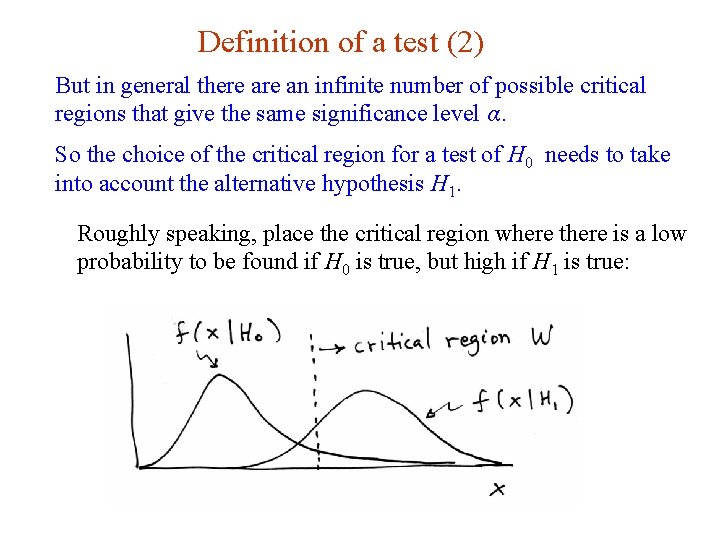
Definition of a test (2) But in general there an infinite number of possible critical regions that give the same significance level α. So the choice of the critical region for a test of H 0 needs to take into account the alternative hypothesis H 1. Roughly speaking, place the critical region where there is a low probability to be found if H 0 is true, but high if H 1 is true: G. Cowan Neutrino Summer School / Mainz, 25, 26 May 2018 24

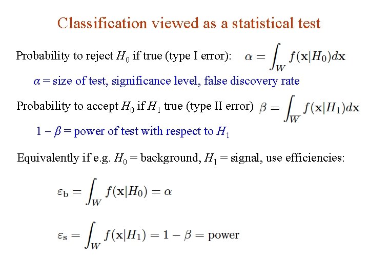
Classification viewed as a statistical test Probability to reject H 0 if true (type I error): α = size of test, significance level, false discovery rate Probability to accept H 0 if H 1 true (type II error): 1 - β = power of test with respect to H 1 Equivalently if e. g. H 0 = background, H 1 = signal, use efficiencies: G. Cowan Neutrino Summer School / Mainz, 25, 26 May 2018 25

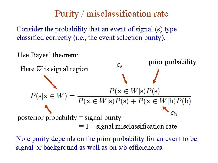
Purity / misclassification rate Consider the probability that an event of signal (s) type classified correctly (i. e. , the event selection purity), Use Bayes’ theorem: Here W is signal region prior probability posterior probability = signal purity = 1 – signal misclassification rate Note purity depends on the prior probability for an event to be signal or background as well as on s/b efficiencies. G. Cowan Neutrino Summer School / Mainz, 25, 26 May 2018 26

Physics context of a statistical test Event Selection: data = individual event; goal is to classify Example: separation of different particle types (electron vs muon) or known event types (ttbar vs QCD multijet). E. g. test H 0 : event is background vs. H 1 : event is signal. Use selected events for further study. Search for New Physics: data = a sample of events. Test null hypothesis H 0 : all events correspond to Standard Model (background only), against the alternative H 1 : events include a type whose existence is not yet established (signal plus background) Many subtle issues here, mainly related to the high standard of proof required to establish presence of a new phenomenon. The optimal statistical test for a search is closely related to that used for event selection. G. Cowan Neutrino Summer School / Mainz, 25, 26 May 2018 27

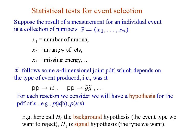
Statistical tests for event selection Suppose the result of a measurement for an individual event is a collection of numbers x 1 = number of muons, x 2 = mean p. T of jets, x 3 = missing energy, . . . follows some n-dimensional joint pdf, which depends on the type of event produced, i. e. , was it For each reaction we consider we will have a hypothesis for the pdf of x , e. g. , p(x|b), p(x|s) E. g. here call H 0 the background hypothesis (the event type we want to reject); H 1 is signal hypothesis (the type we want). G. Cowan Neutrino Summer School / Mainz, 25, 26 May 2018 28

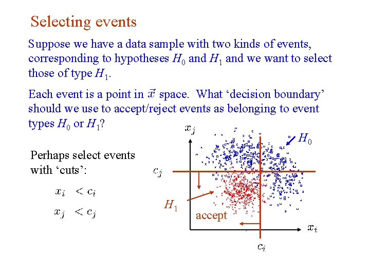
Selecting events Suppose we have a data sample with two kinds of events, corresponding to hypotheses H 0 and H 1 and we want to select those of type H 1. Each event is a point in space. What ‘decision boundary’ should we use to accept/reject events as belonging to event types H 0 or H 1? H 0 Perhaps select events with ‘cuts’: H 1 G. Cowan accept Neutrino Summer School / Mainz, 25, 26 May 2018 29

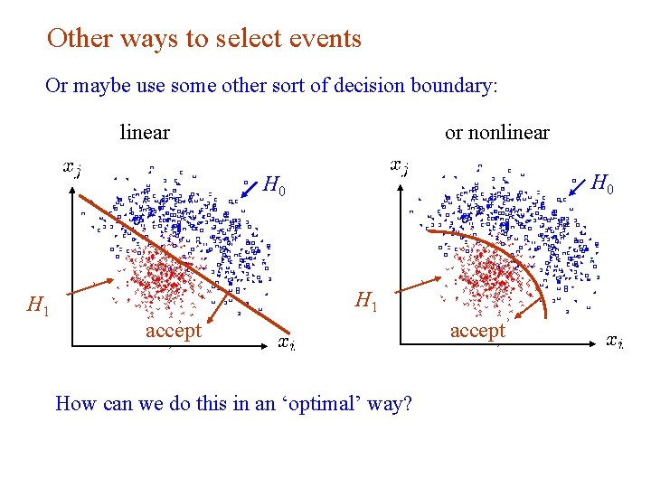
Other ways to select events Or maybe use some other sort of decision boundary: linear or nonlinear H 0 H 1 accept How can we do this in an ‘optimal’ way? G. Cowan Neutrino Summer School / Mainz, 25, 26 May 2018 30

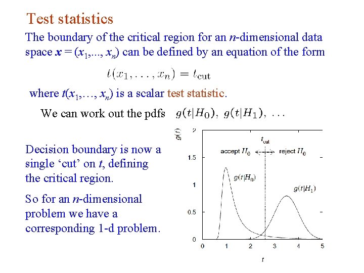
Test statistics The boundary of the critical region for an n-dimensional data space x = (x 1, . . . , xn) can be defined by an equation of the form where t(x 1, …, xn) is a scalar test statistic. We can work out the pdfs Decision boundary is now a single ‘cut’ on t, defining the critical region. So for an n-dimensional problem we have a corresponding 1 -d problem. G. Cowan Neutrino Summer School / Mainz, 25, 26 May 2018 31

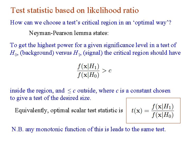
Test statistic based on likelihood ratio How can we choose a test’s critical region in an ‘optimal way’? Neyman-Pearson lemma states: To get the highest power for a given significance level in a test of H 0, (background) versus H 1, (signal) the critical region should have inside the region, and ≤ c outside, where c is a constant chosen to give a test of the desired size. Equivalently, optimal scalar test statistic is N. B. any monotonic function of this is leads to the same test. G. Cowan Neutrino Summer School / Mainz, 25, 26 May 2018 32

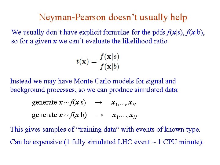
Neyman-Pearson doesn’t usually help We usually don’t have explicit formulae for the pdfs f (x|s), f (x|b), so for a given x we can’t evaluate the likelihood ratio Instead we may have Monte Carlo models for signal and background processes, so we can produce simulated data: generate x ~ f (x|s) → x 1, . . . , x. N generate x ~ f (x|b) → x 1, . . . , x. N This gives samples of “training data” with events of known type. Can be expensive (1 fully simulated LHC event ~ 1 CPU minute). G. Cowan Neutrino Summer School / Mainz, 25, 26 May 2018 33

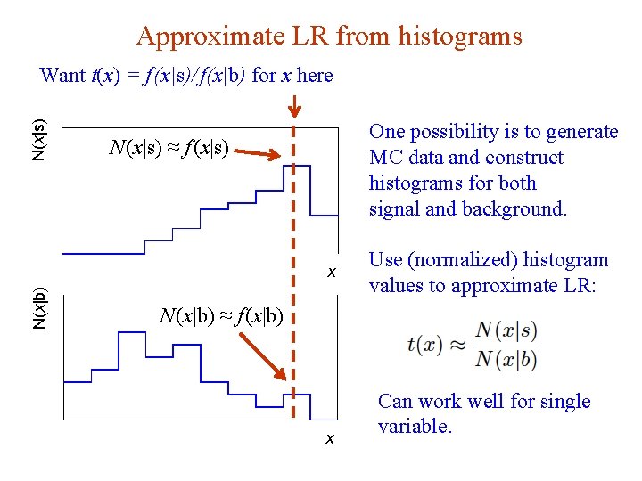
Approximate LR from histograms N(x|s) Want t(x) = f (x|s)/ f(x|b) for x here One possibility is to generate MC data and construct histograms for both signal and background. N (x|s) ≈ f (x|s) N(x|b) x N (x|b) ≈ f (x|b) x G. Cowan Use (normalized) histogram values to approximate LR: Can work well for single variable. Neutrino Summer School / Mainz, 25, 26 May 2018 34

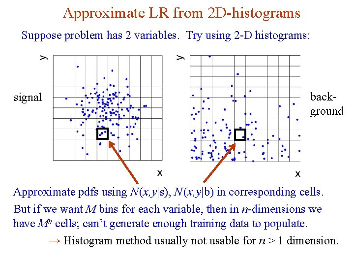
Approximate LR from 2 D-histograms Suppose problem has 2 variables. Try using 2 -D histograms: background signal Approximate pdfs using N (x, y|s), N (x, y|b) in corresponding cells. But if we want M bins for each variable, then in n-dimensions we have Mn cells; can’t generate enough training data to populate. → Histogram method usually not usable for n > 1 dimension. G. Cowan Neutrino Summer School / Mainz, 25, 26 May 2018 35

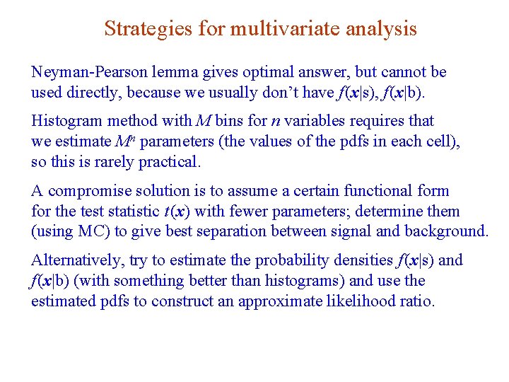
Strategies for multivariate analysis Neyman-Pearson lemma gives optimal answer, but cannot be used directly, because we usually don’t have f (x|s), f (x|b). Histogram method with M bins for n variables requires that we estimate Mn parameters (the values of the pdfs in each cell), so this is rarely practical. A compromise solution is to assume a certain functional form for the test statistic t (x) with fewer parameters; determine them (using MC) to give best separation between signal and background. Alternatively, try to estimate the probability densities f (x|s) and f (x|b) (with something better than histograms) and use the estimated pdfs to construct an approximate likelihood ratio. G. Cowan Neutrino Summer School / Mainz, 25, 26 May 2018 36

Multivariate methods Many new (and some old) methods esp. from Machine Learning: Fisher discriminant (Deep) neural networks Kernel density methods Support Vector Machines Decision trees Boosting Bagging This is a large topic -- see e. g. lectures http: //www. pp. rhul. ac. uk/~cowan/stat_2. pdf (from around p 38) and references therein. G. Cowan Neutrino Summer School / Mainz, 25, 26 May 2018 37

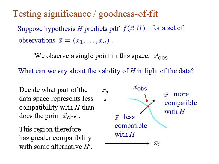
Testing significance / goodness-of-fit Suppose hypothesis H predicts pdf for a set of observations We observe a single point in this space: What can we say about the validity of H in light of the data? Decide what part of the data space represents less compatibility with H than does the point This region therefore has greater compatibility with some alternative Hʹ. G. Cowan less compatible with H Neutrino Summer School / Mainz, 25, 26 May 2018 more compatible with H 38

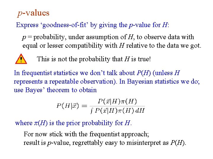
p-values Express ‘goodness-of-fit’ by giving the p-value for H: p = probability, under assumption of H, to observe data with equal or lesser compatibility with H relative to the data we got. This is not the probability that H is true! In frequentist statistics we don’t talk about P(H) (unless H represents a repeatable observation). In Bayesian statistics we do; use Bayes’ theorem to obtain where π(H) is the prior probability for H. For now stick with the frequentist approach; result is p-value, regrettably easy to misinterpret as P(H). G. Cowan Neutrino Summer School / Mainz, 25, 26 May 2018 39

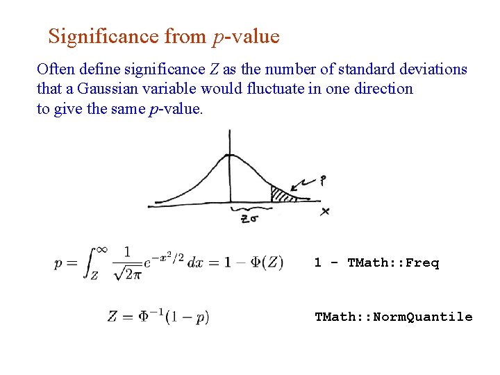
Significance from p-value Often define significance Z as the number of standard deviations that a Gaussian variable would fluctuate in one direction to give the same p-value. 1 - TMath: : Freq TMath: : Norm. Quantile G. Cowan Neutrino Summer School / Mainz, 25, 26 May 2018 40

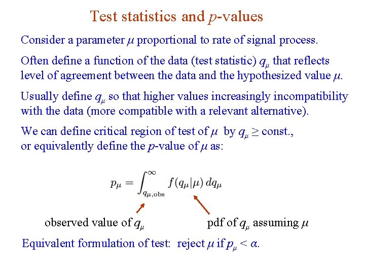
Test statistics and p-values Consider a parameter μ proportional to rate of signal process. Often define a function of the data (test statistic) qμ that reflects level of agreement between the data and the hypothesized value μ. Usually define qμ so that higher values increasingly incompatibility with the data (more compatible with a relevant alternative). We can define critical region of test of μ by qμ ≥ const. , or equivalently define the p-value of μ as: observed value of qμ pdf of qμ assuming μ Equivalent formulation of test: reject μ if pμ < α. G. Cowan Neutrino Summer School / Mainz, 25, 26 May 2018 41

Confidence interval from inversion of a test Carry out a test of size α for all values of μ. The values that are not rejected constitute a confidence interval for μ at confidence level CL = 1 – α. The confidence interval will by construction contain the true value of μ with probability of at least 1 – α. The interval will cover the true value of μ with probability ≥ 1 - α. Equivalently, the parameter values in the confidence interval have p-values of at least α. To find edge of interval (the “limit”), set pμ = α and solve for μ. G. Cowan Neutrino Summer School / Mainz, 25, 26 May 2018 42

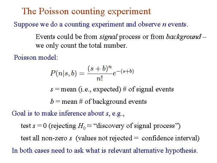
The Poisson counting experiment Suppose we do a counting experiment and observe n events. Events could be from signal process or from background – we only count the total number. Poisson model: s = mean (i. e. , expected) # of signal events b = mean # of background events Goal is to make inference about s, e. g. , test s = 0 (rejecting H 0 ≈ “discovery of signal process”) test all non-zero s (values not rejected = confidence interval) In both cases need to ask what is relevant alternative hypothesis. G. Cowan Neutrino Summer School / Mainz, 25, 26 May 2018 43

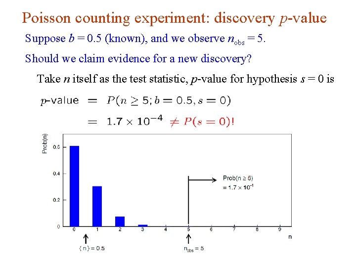
Poisson counting experiment: discovery p-value Suppose b = 0. 5 (known), and we observe nobs = 5. Should we claim evidence for a new discovery? Take n itself as the test statistic, p-value for hypothesis s = 0 is G. Cowan Neutrino Summer School / Mainz, 25, 26 May 2018 44

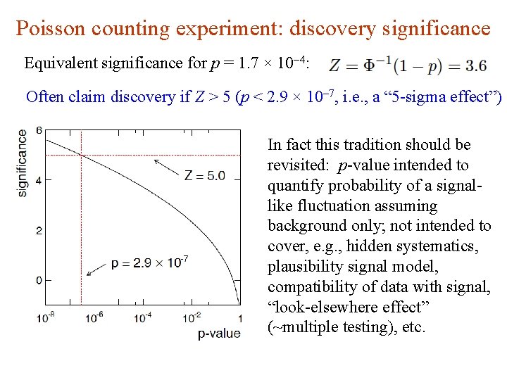
Poisson counting experiment: discovery significance Equivalent significance for p = 1. 7 × 10 -4: Often claim discovery if Z > 5 (p < 2. 9 × 10 -7, i. e. , a “ 5 -sigma effect”) In fact this tradition should be revisited: p-value intended to quantify probability of a signallike fluctuation assuming background only; not intended to cover, e. g. , hidden systematics, plausibility signal model, compatibility of data with signal, “look-elsewhere effect” (~multiple testing), etc. G. Cowan Neutrino Summer School / Mainz, 25, 26 May 2018 45

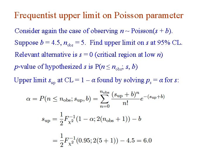
Frequentist upper limit on Poisson parameter Consider again the case of observing n ~ Poisson(s + b). Suppose b = 4. 5, nobs = 5. Find upper limit on s at 95% CL. Relevant alternative is s = 0 (critical region at low n) p-value of hypothesized s is P(n ≤ nobs; s, b) Upper limit sup at CL = 1 – α found by solving ps = α for s: G. Cowan Neutrino Summer School / Mainz, 25, 26 May 2018 46

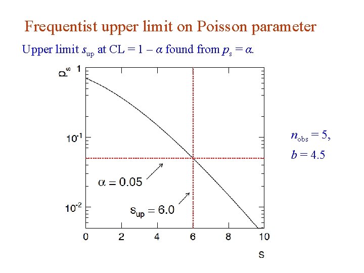
Frequentist upper limit on Poisson parameter Upper limit sup at CL = 1 – α found from ps = α. nobs = 5, b = 4. 5 G. Cowan Neutrino Summer School / Mainz, 25, 26 May 2018 47

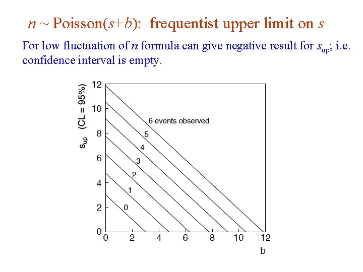
n ~ Poisson(s+b): frequentist upper limit on s For low fluctuation of n formula can give negative result for sup; i. e. confidence interval is empty. G. Cowan Neutrino Summer School / Mainz, 25, 26 May 2018 48

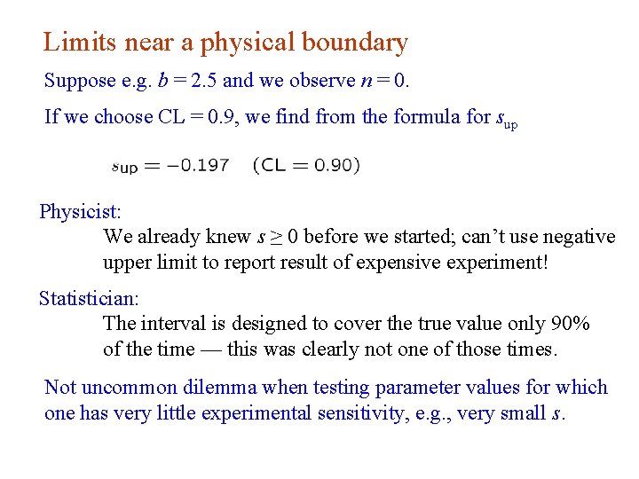
Limits near a physical boundary Suppose e. g. b = 2. 5 and we observe n = 0. If we choose CL = 0. 9, we find from the formula for sup Physicist: We already knew s ≥ 0 before we started; can’t use negative upper limit to report result of expensive experiment! Statistician: The interval is designed to cover the true value only 90% of the time — this was clearly not one of those times. Not uncommon dilemma when testing parameter values for which one has very little experimental sensitivity, e. g. , very small s. G. Cowan Neutrino Summer School / Mainz, 25, 26 May 2018 49

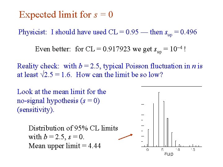
Expected limit for s = 0 Physicist: I should have used CL = 0. 95 — then sup = 0. 496 Even better: for CL = 0. 917923 we get sup = 10 -4 ! Reality check: with b = 2. 5, typical Poisson fluctuation in n is at least √ 2. 5 = 1. 6. How can the limit be so low? Look at the mean limit for the no-signal hypothesis (s = 0) (sensitivity). Distribution of 95% CL limits with b = 2. 5, s = 0. Mean upper limit = 4. 44 G. Cowan Neutrino Summer School / Mainz, 25, 26 May 2018 50

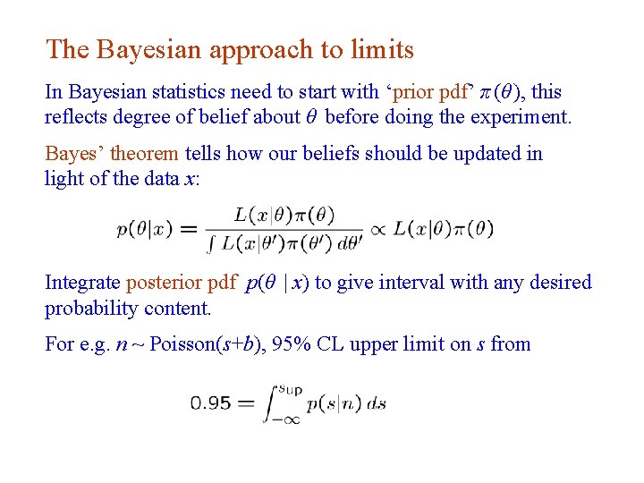
The Bayesian approach to limits In Bayesian statistics need to start with ‘prior pdf’ π (θ ), this reflects degree of belief about θ before doing the experiment. Bayes’ theorem tells how our beliefs should be updated in light of the data x: Integrate posterior pdf p(θ | x) to give interval with any desired probability content. For e. g. n ~ Poisson(s+b), 95% CL upper limit on s from G. Cowan Neutrino Summer School / Mainz, 25, 26 May 2018 51

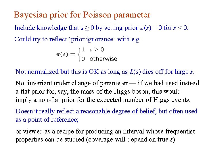
Bayesian prior for Poisson parameter Include knowledge that s ≥ 0 by setting prior π (s) = 0 for s < 0. Could try to reflect ‘prior ignorance’ with e. g. Not normalized but this is OK as long as L(s) dies off for large s. Not invariant under change of parameter — if we had used instead a flat prior for, say, the mass of the Higgs boson, this would imply a non-flat prior for the expected number of Higgs events. Doesn’t really reflect a reasonable degree of belief, but often used as a point of reference; or viewed as a recipe for producing an interval whose frequentist properties can be studied (coverage will depend on true s). G. Cowan Neutrino Summer School / Mainz, 25, 26 May 2018 52

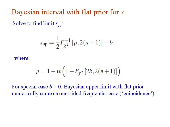
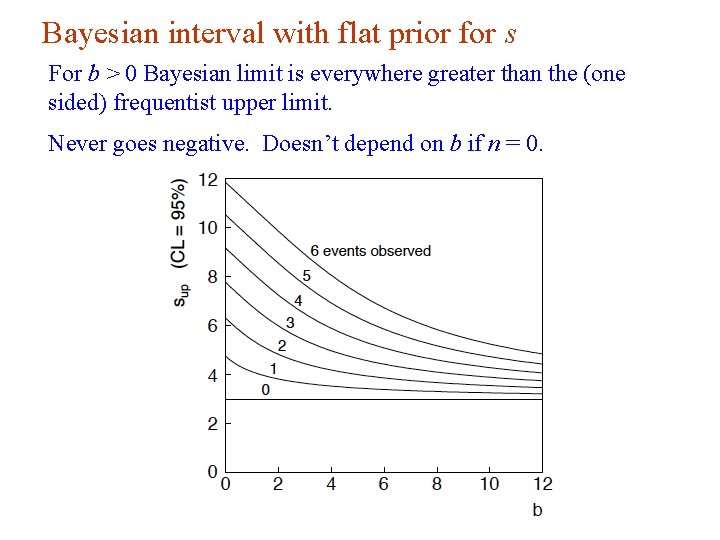
Bayesian interval with flat prior for s Solve to find limit sup: where For special case b = 0, Bayesian upper limit with flat prior numerically same as one-sided frequentist case (‘coincidence’). G. Cowan Neutrino Summer School / Mainz, 25, 26 May 2018 53

Bayesian interval with flat prior for s For b > 0 Bayesian limit is everywhere greater than the (one sided) frequentist upper limit. Never goes negative. Doesn’t depend on b if n = 0. G. Cowan Neutrino Summer School / Mainz, 25, 26 May 2018 54

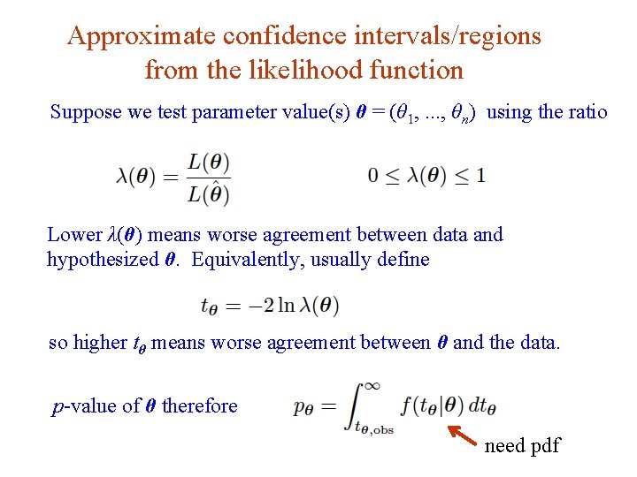
Approximate confidence intervals/regions from the likelihood function Suppose we test parameter value(s) θ = (θ 1, . . . , θn) using the ratio Lower λ(θ) means worse agreement between data and hypothesized θ. Equivalently, usually define so higher tθ means worse agreement between θ and the data. p-value of θ therefore G. Cowan Neutrino Summer School / Mainz, 25, 26 May 2018 need pdf 55

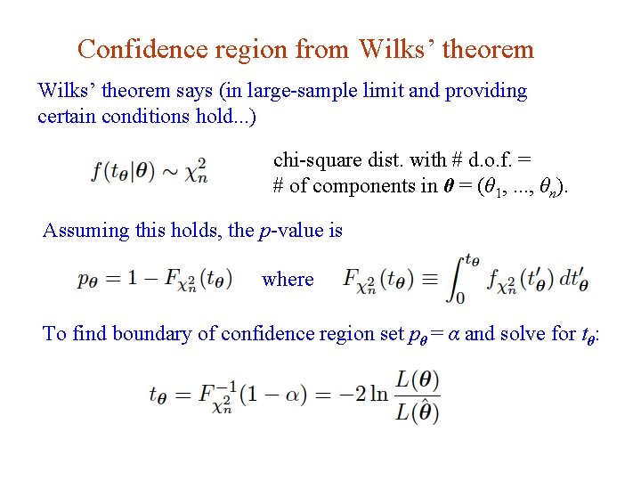
Confidence region from Wilks’ theorem says (in large-sample limit and providing certain conditions hold. . . ) chi-square dist. with # d. o. f. = # of components in θ = (θ 1, . . . , θn). Assuming this holds, the p-value is where To find boundary of confidence region set pθ = α and solve for tθ: G. Cowan Neutrino Summer School / Mainz, 25, 26 May 2018 56

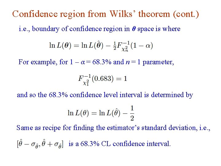
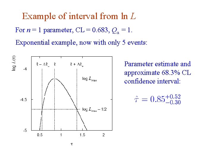
Confidence region from Wilks’ theorem (cont. ) i. e. , boundary of confidence region in θ space is where For example, for 1 – α = 68. 3% and n = 1 parameter, and so the 68. 3% confidence level interval is determined by Same as recipe for finding the estimator’s standard deviation, i. e. , is a 68. 3% CL confidence interval. G. Cowan Neutrino Summer School / Mainz, 25, 26 May 2018 57

Example of interval from ln L For n = 1 parameter, CL = 0. 683, Qα = 1. Exponential example, now with only 5 events: Parameter estimate and approximate 68. 3% CL confidence interval: G. Cowan Neutrino Summer School / Mainz, 25, 26 May 2018 58

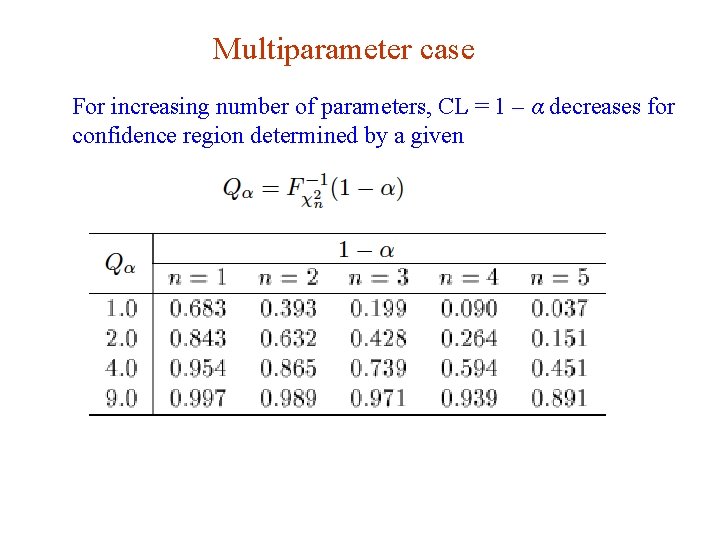
Multiparameter case For increasing number of parameters, CL = 1 – α decreases for confidence region determined by a given G. Cowan Neutrino Summer School / Mainz, 25, 26 May 2018 59

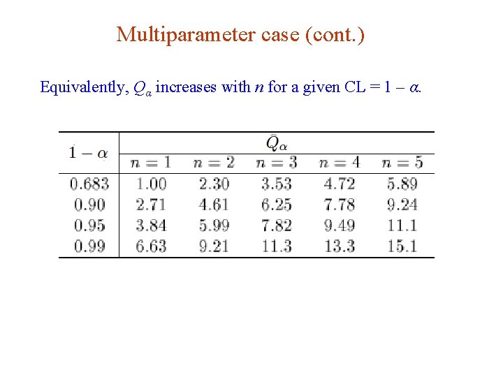
Multiparameter case (cont. ) Equivalently, Qα increases with n for a given CL = 1 – α. G. Cowan Neutrino Summer School / Mainz, 25, 26 May 2018 60

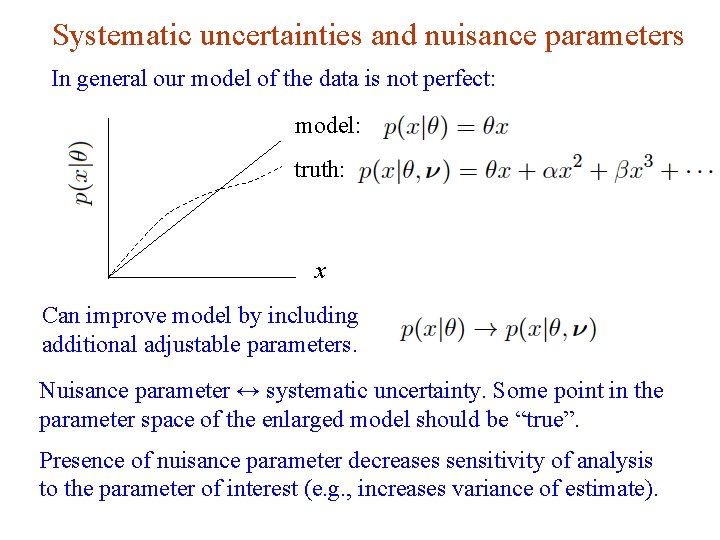
Systematic uncertainties and nuisance parameters In general our model of the data is not perfect: model: truth: x Can improve model by including additional adjustable parameters. Nuisance parameter ↔ systematic uncertainty. Some point in the parameter space of the enlarged model should be “true”. Presence of nuisance parameter decreases sensitivity of analysis to the parameter of interest (e. g. , increases variance of estimate). G. Cowan Neutrino Summer School / Mainz, 25, 26 May 2018 61

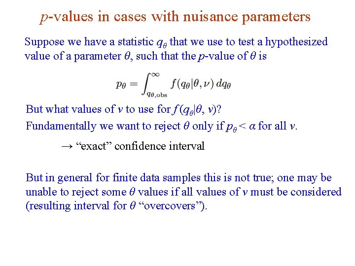
p-values in cases with nuisance parameters Suppose we have a statistic qθ that we use to test a hypothesized value of a parameter θ, such that the p-value of θ is But what values of ν to use for f (qθ|θ, ν)? Fundamentally we want to reject θ only if pθ < α for all ν. → “exact” confidence interval But in general for finite data samples this is not true; one may be unable to reject some θ values if all values of ν must be considered (resulting interval for θ “overcovers”). G. Cowan Neutrino Summer School / Mainz, 25, 26 May 2018 62

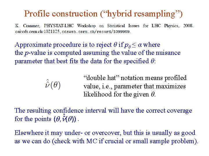
Profile construction (“hybrid resampling”) Approximate procedure is to reject θ if pθ ≤ α where the p-value is computed assuming the value of the nuisance parameter that best fits the data for the specified θ: “double hat” notation means profiled value, i. e. , parameter that maximizes likelihood for the given θ. The resulting confidence interval will have the correct coverage. for the points Elsewhere it may under- or overcover, but this is usually as good as we can do (check with MC if crucial or small sample problem). G. Cowan Neutrino Summer School / Mainz, 25, 26 May 2018 63

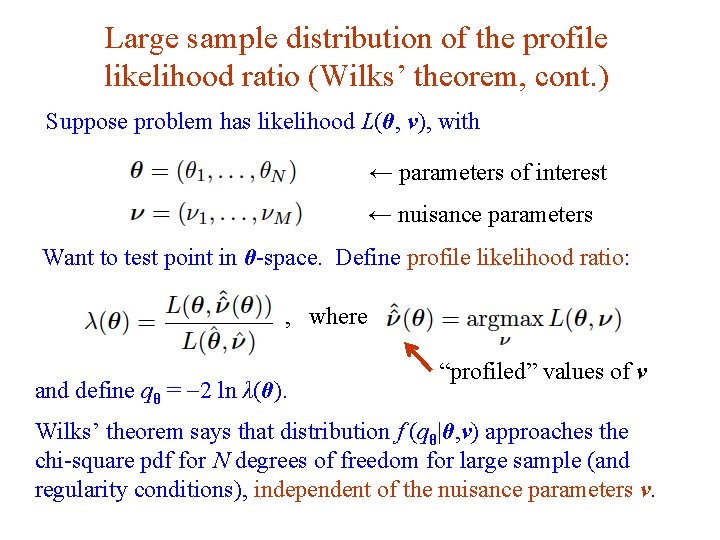
Large sample distribution of the profile likelihood ratio (Wilks’ theorem, cont. ) Suppose problem has likelihood L(θ, ν), with ← parameters of interest ← nuisance parameters Want to test point in θ-space. Define profile likelihood ratio: , where and define qθ = -2 ln λ(θ). “profiled” values of ν Wilks’ theorem says that distribution f (qθ|θ, ν) approaches the chi-square pdf for N degrees of freedom for large sample (and regularity conditions), independent of the nuisance parameters ν. G. Cowan Neutrino Summer School / Mainz, 25, 26 May 2018 64

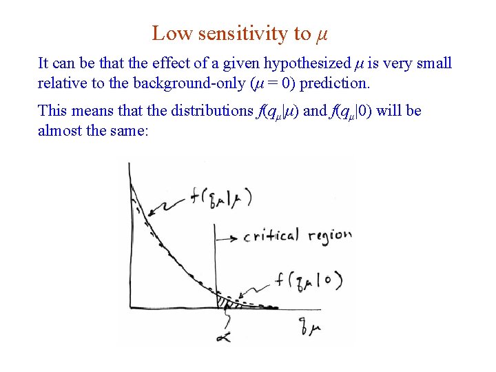
Low sensitivity to μ It can be that the effect of a given hypothesized μ is very small relative to the background-only (μ = 0) prediction. This means that the distributions f(qμ|μ) and f(qμ|0) will be almost the same: G. Cowan Neutrino Summer School / Mainz, 25, 26 May 2018 65

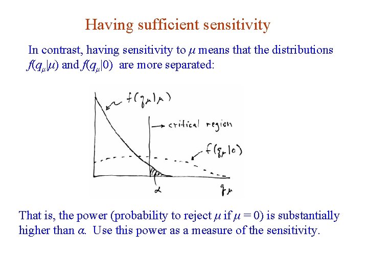
Having sufficient sensitivity In contrast, having sensitivity to μ means that the distributions f(qμ|μ) and f(qμ|0) are more separated: That is, the power (probability to reject μ if μ = 0) is substantially higher than α. Use this power as a measure of the sensitivity. G. Cowan Neutrino Summer School / Mainz, 25, 26 May 2018 66

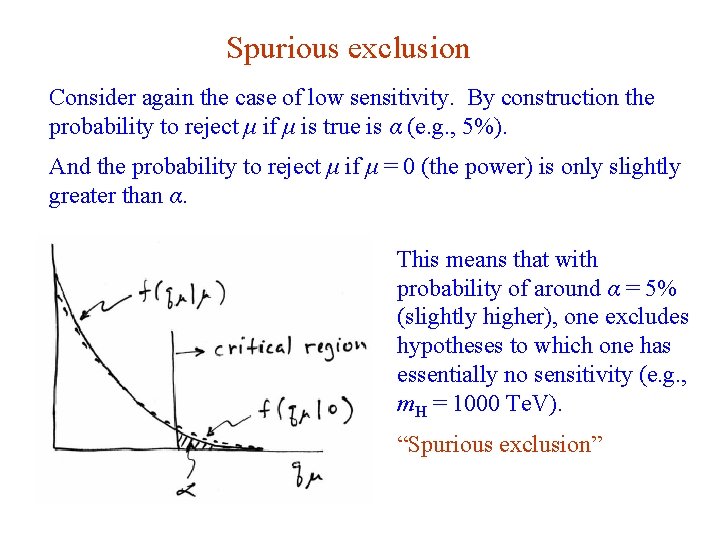
Spurious exclusion Consider again the case of low sensitivity. By construction the probability to reject μ if μ is true is α (e. g. , 5%). And the probability to reject μ if μ = 0 (the power) is only slightly greater than α. This means that with probability of around α = 5% (slightly higher), one excludes hypotheses to which one has essentially no sensitivity (e. g. , m. H = 1000 Te. V). “Spurious exclusion” G. Cowan Neutrino Summer School / Mainz, 25, 26 May 2018 67

Ways of addressing spurious exclusion The problem of excluding parameter values to which one has no sensitivity known for a long time; see e. g. , In the 1990 s this was re-examined for the LEP Higgs search by Alex Read and others and led to the “CLs” procedure for upper limits. Unified intervals also effectively reduce spurious exclusion by the particular choice of critical region. G. Cowan Neutrino Summer School / Mainz, 25, 26 May 2018 68

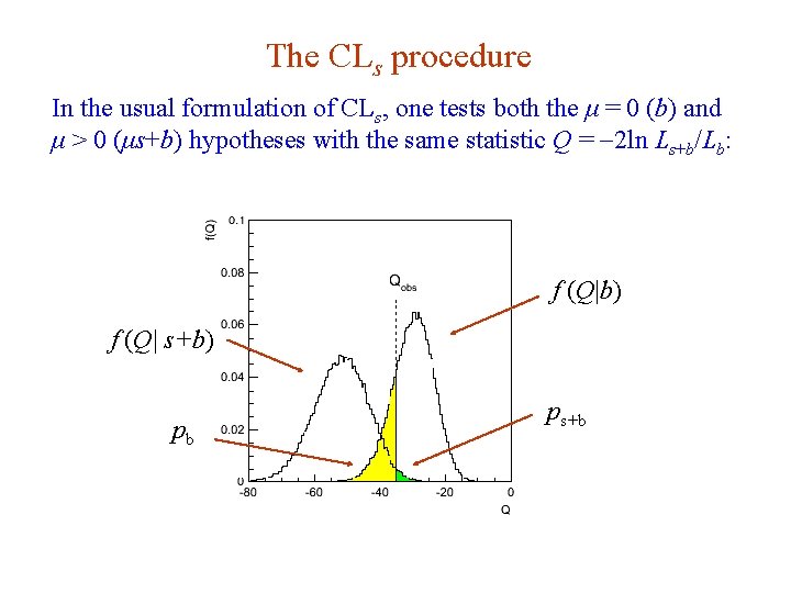
The CLs procedure In the usual formulation of CLs, one tests both the μ = 0 (b) and μ > 0 (μs+b) hypotheses with the same statistic Q = -2 ln Ls+b/Lb: f (Q|b) f (Q| s+b) pb G. Cowan ps+b Neutrino Summer School / Mainz, 25, 26 May 2018 69

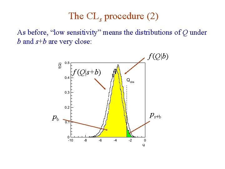
The CLs procedure (2) As before, “low sensitivity” means the distributions of Q under b and s+b are very close: f (Q|b) f (Q|s+b) pb G. Cowan ps+b Neutrino Summer School / Mainz, 25, 26 May 2018 70

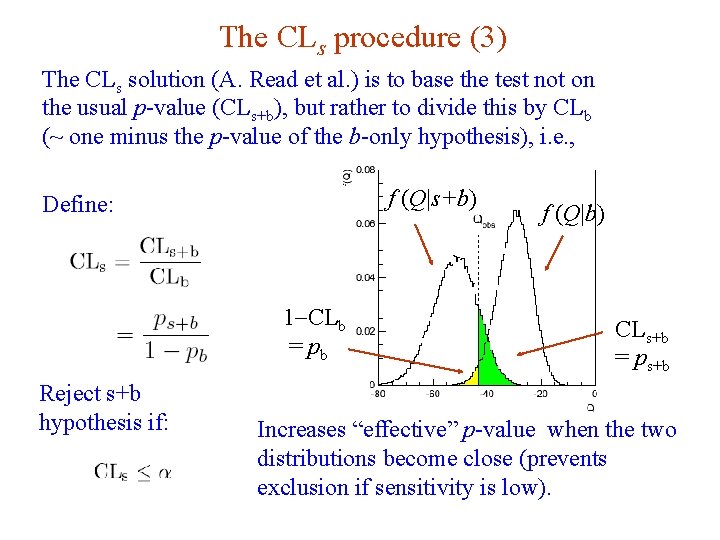
The CLs procedure (3) The CLs solution (A. Read et al. ) is to base the test not on the usual p-value (CLs+b), but rather to divide this by CLb (~ one minus the p-value of the b-only hypothesis), i. e. , f (Q|s+b) Define: f (Q|b) 1 -CLb = pb Reject s+b hypothesis if: G. Cowan CLs+b = ps+b Increases “effective” p-value when the two distributions become close (prevents exclusion if sensitivity is low). Neutrino Summer School / Mainz, 25, 26 May 2018 71

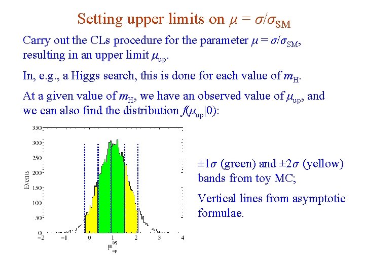
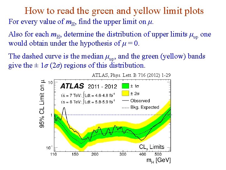
Setting upper limits on μ = σ/σSM Carry out the CLs procedure for the parameter μ = σ/σSM, resulting in an upper limit μup. In, e. g. , a Higgs search, this is done for each value of m. H. At a given value of m. H, we have an observed value of μup, and we can also find the distribution f(μup|0): ± 1σ (green) and ± 2σ (yellow) bands from toy MC; Vertical lines from asymptotic formulae. G. Cowan Neutrino Summer School / Mainz, 25, 26 May 2018 72

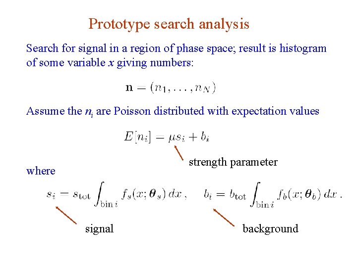
Prototype search analysis Search for signal in a region of phase space; result is histogram of some variable x giving numbers: Assume the ni are Poisson distributed with expectation values strength parameter where signal G. Cowan background Neutrino Summer School / Mainz, 25, 26 May 2018 73

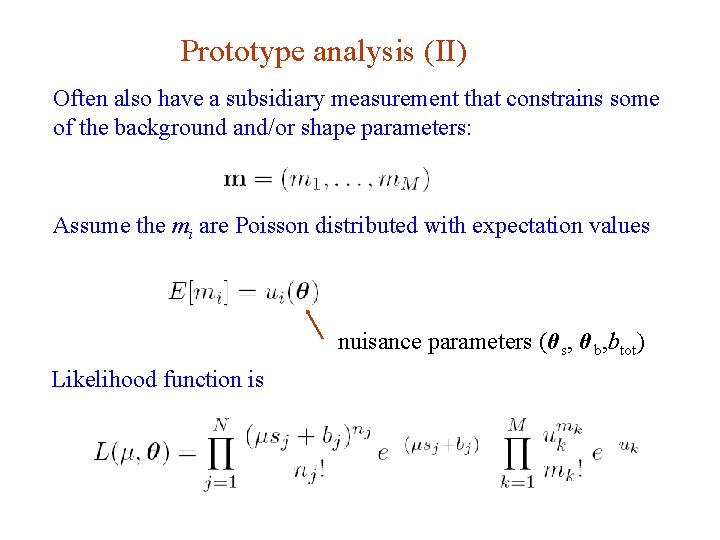
Prototype analysis (II) Often also have a subsidiary measurement that constrains some of the background and/or shape parameters: Assume the mi are Poisson distributed with expectation values nuisance parameters (θ s, θ b, btot) Likelihood function is G. Cowan Neutrino Summer School / Mainz, 25, 26 May 2018 74

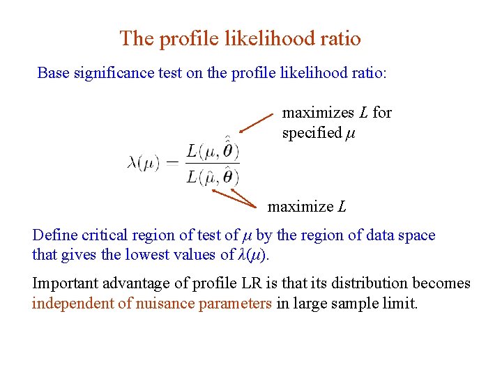
The profile likelihood ratio Base significance test on the profile likelihood ratio: maximizes L for specified μ maximize L Define critical region of test of μ by the region of data space that gives the lowest values of λ(μ). Important advantage of profile LR is that its distribution becomes independent of nuisance parameters in large sample limit. G. Cowan Neutrino Summer School / Mainz, 25, 26 May 2018 75

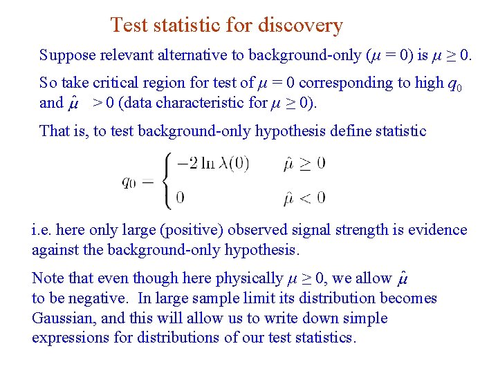
Test statistic for discovery Suppose relevant alternative to background-only (μ = 0) is μ ≥ 0. So take critical region for test of μ = 0 corresponding to high q 0 and > 0 (data characteristic for μ ≥ 0). That is, to test background-only hypothesis define statistic i. e. here only large (positive) observed signal strength is evidence against the background-only hypothesis. Note that even though here physically μ ≥ 0, we allow to be negative. In large sample limit its distribution becomes Gaussian, and this will allow us to write down simple expressions for distributions of our test statistics. G. Cowan Neutrino Summer School / Mainz, 25, 26 May 2018 76

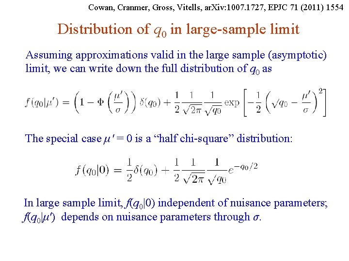
Cowan, Cranmer, Gross, Vitells, ar. Xiv: 1007. 1727, EPJC 71 (2011) 1554 Distribution of q 0 in large-sample limit Assuming approximations valid in the large sample (asymptotic) limit, we can write down the full distribution of q 0 as The special case μ′ = 0 is a “half chi-square” distribution: In large sample limit, f(q 0|0) independent of nuisance parameters; f(q 0|μ′) depends on nuisance parameters through σ. G. Cowan Neutrino Summer School / Mainz, 25, 26 May 2018 77

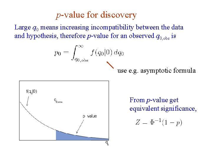
p-value for discovery Large q 0 means increasing incompatibility between the data and hypothesis, therefore p-value for an observed q 0, obs is use e. g. asymptotic formula From p-value get equivalent significance, G. Cowan Neutrino Summer School / Mainz, 25, 26 May 2018 78

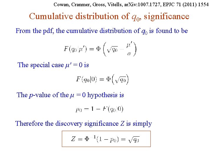
Cowan, Cranmer, Gross, Vitells, ar. Xiv: 1007. 1727, EPJC 71 (2011) 1554 Cumulative distribution of q 0, significance From the pdf, the cumulative distribution of q 0 is found to be The special case μ′ = 0 is The p-value of the μ = 0 hypothesis is Therefore the discovery significance Z is simply G. Cowan Neutrino Summer School / Mainz, 25, 26 May 2018 79

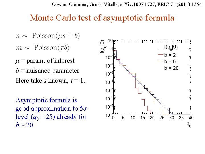
Cowan, Cranmer, Gross, Vitells, ar. Xiv: 1007. 1727, EPJC 71 (2011) 1554 Monte Carlo test of asymptotic formula μ = param. of interest b = nuisance parameter Here take s known, τ = 1. Asymptotic formula is good approximation to 5σ level (q 0 = 25) already for b ~ 20. G. Cowan Neutrino Summer School / Mainz, 25, 26 May 2018 80

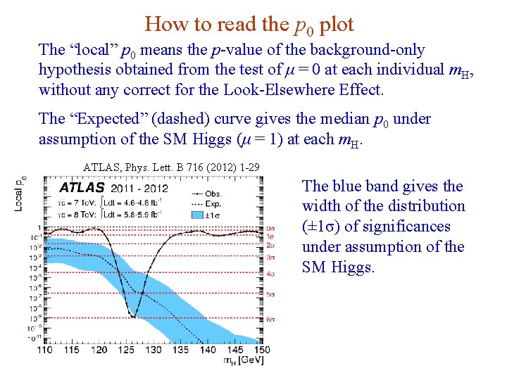
How to read the p 0 plot The “local” p 0 means the p-value of the background-only hypothesis obtained from the test of μ = 0 at each individual m. H, without any correct for the Look-Elsewhere Effect. The “Expected” (dashed) curve gives the median p 0 under assumption of the SM Higgs (μ = 1) at each m. H. ATLAS, Phys. Lett. B 716 (2012) 1 -29 The blue band gives the width of the distribution (± 1σ) of significances under assumption of the SM Higgs. G. Cowan Neutrino Summer School / Mainz, 25, 26 May 2018 81

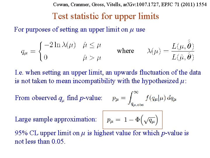
Cowan, Cranmer, Gross, Vitells, ar. Xiv: 1007. 1727, EPJC 71 (2011) 1554 Test statistic for upper limits For purposes of setting an upper limit on μ use where I. e. when setting an upper limit, an upwards fluctuation of the data is not taken to mean incompatibility with the hypothesized μ: From observed qμ find p-value: Large sample approximation: 95% CL upper limit on μ is highest value for which p-value is not less than 0. 05. G. Cowan Neutrino Summer School / Mainz, 25, 26 May 2018 82

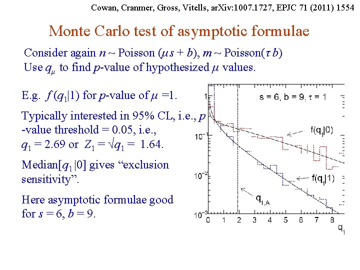
Cowan, Cranmer, Gross, Vitells, ar. Xiv: 1007. 1727, EPJC 71 (2011) 1554 Monte Carlo test of asymptotic formulae Consider again n ~ Poisson (μs + b), m ~ Poisson(τ b) Use qμ to find p-value of hypothesized μ values. E. g. f (q 1|1) for p-value of μ =1. Typically interested in 95% CL, i. e. , p -value threshold = 0. 05, i. e. , q 1 = 2. 69 or Z 1 = √q 1 = 1. 64. Median[q 1 |0] gives “exclusion sensitivity”. Here asymptotic formulae good for s = 6, b = 9. G. Cowan Neutrino Summer School / Mainz, 25, 26 May 2018 83

How to read the green and yellow limit plots For every value of m. H, find the upper limit on μ. Also for each m. H, determine the distribution of upper limits μup one would obtain under the hypothesis of μ = 0. The dashed curve is the median μup, and the green (yellow) bands give the ± 1σ (2σ) regions of this distribution. ATLAS, Phys. Lett. B 716 (2012) 1 -29 G. Cowan Neutrino Summer School / Mainz, 25, 26 May 2018 84

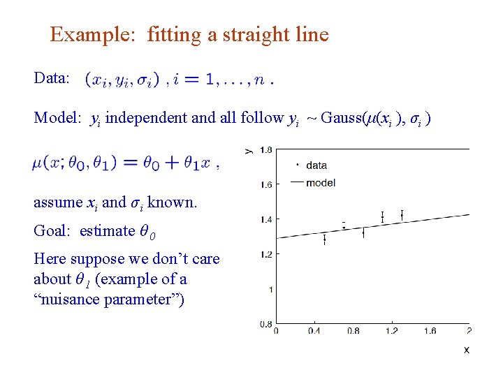
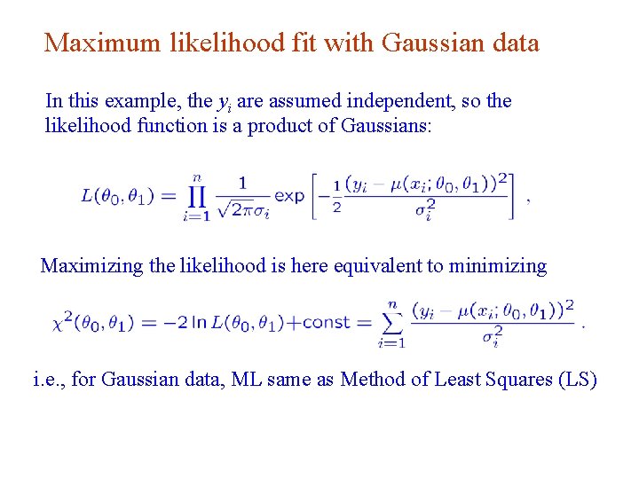
Example: fitting a straight line Data: Model: yi independent and all follow yi ~ Gauss(μ(xi ), σi ) assume xi and σ i known. Goal: estimate θ 0 Here suppose we don’t care about θ 1 (example of a “nuisance parameter”) G. Cowan Neutrino Summer School / Mainz, 25, 26 May 2018 85

Maximum likelihood fit with Gaussian data In this example, the yi are assumed independent, so the likelihood function is a product of Gaussians: Maximizing the likelihood is here equivalent to minimizing i. e. , for Gaussian data, ML same as Method of Least Squares (LS) G. Cowan Neutrino Summer School / Mainz, 25, 26 May 2018 86

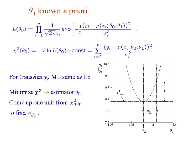
θ 1 known a priori For Gaussian yi, ML same as LS Minimize χ 2 → estimator Come up one unit from to find G. Cowan Neutrino Summer School / Mainz, 25, 26 May 2018 87

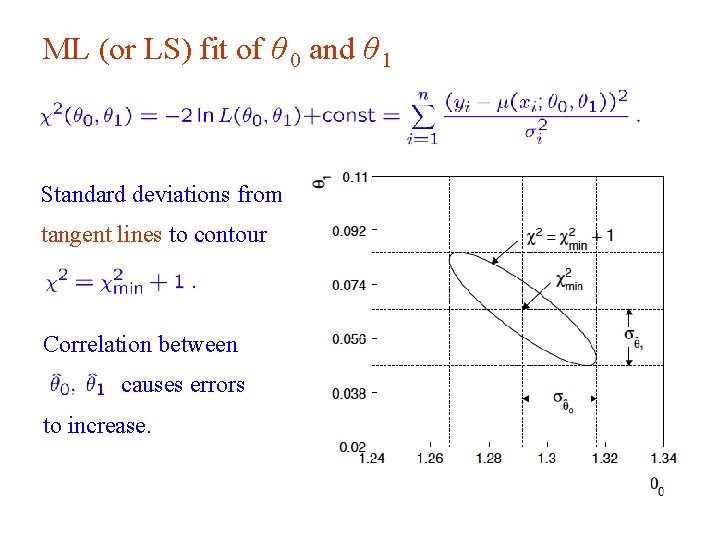
ML (or LS) fit of θ 0 and θ 1 Standard deviations from tangent lines to contour Correlation between causes errors to increase. G. Cowan Neutrino Summer School / Mainz, 25, 26 May 2018 88

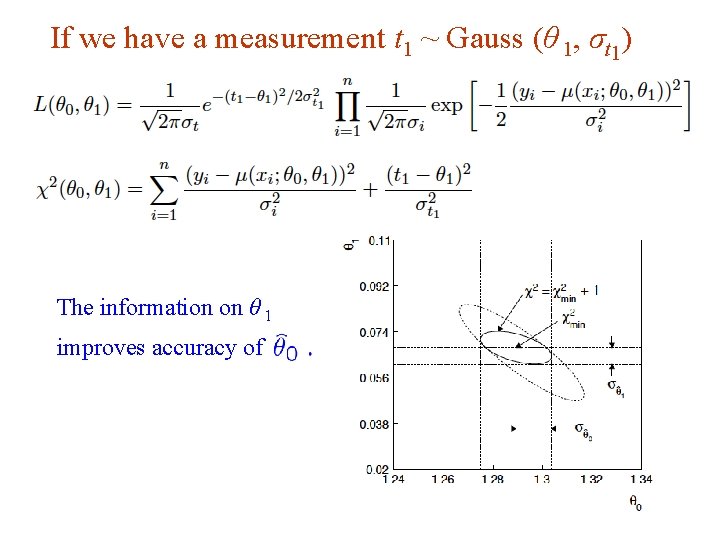
If we have a measurement t 1 ~ Gauss (θ 1, σt 1) The information on θ 1 improves accuracy of G. Cowan Neutrino Summer School / Mainz, 25, 26 May 2018 89

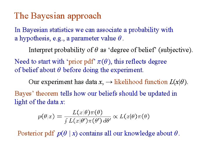
The Bayesian approach In Bayesian statistics we can associate a probability with a hypothesis, e. g. , a parameter value θ. Interpret probability of θ as ‘degree of belief’ (subjective). Need to start with ‘prior pdf’ π (θ ), this reflects degree of belief about θ before doing the experiment. Our experiment has data x, → likelihood function L(x|θ ). Bayes’ theorem tells how our beliefs should be updated in light of the data x: Posterior pdf p(θ | x) contains all our knowledge about θ. G. Cowan Neutrino Summer School / Mainz, 25, 26 May 2018 Lecture 13 page 90

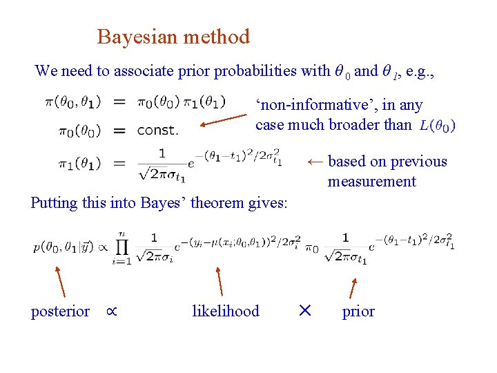
Bayesian method We need to associate prior probabilities with θ 0 and θ 1, e. g. , ‘non-informative’, in any case much broader than ← based on previous measurement Putting this into Bayes’ theorem gives: posterior G. Cowan ∝ likelihood ✕ prior Neutrino Summer School / Mainz, 25, 26 May 2018 91

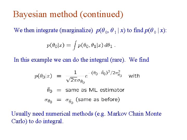
Bayesian method (continued) We then integrate (marginalize) p(θ 0, θ 1 | x) to find p(θ 0 | x): In this example we can do the integral (rare). We find Usually need numerical methods (e. g. Markov Chain Monte Carlo) to do integral. G. Cowan Neutrino Summer School / Mainz, 25, 26 May 2018 92

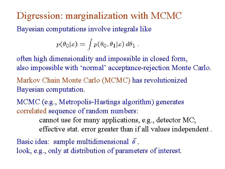
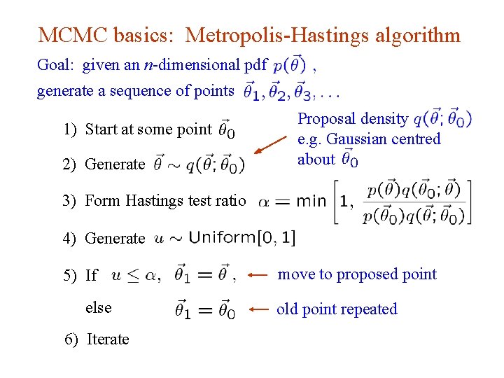
Digression: marginalization with MCMC Bayesian computations involve integrals like often high dimensionality and impossible in closed form, also impossible with ‘normal’ acceptance-rejection Monte Carlo. Markov Chain Monte Carlo (MCMC) has revolutionized Bayesian computation. MCMC (e. g. , Metropolis-Hastings algorithm) generates correlated sequence of random numbers: cannot use for many applications, e. g. , detector MC; effective stat. error greater than if all values independent. Basic idea: sample multidimensional look, e. g. , only at distribution of parameters of interest. G. Cowan Neutrino Summer School / Mainz, 25, 26 May 2018 93

MCMC basics: Metropolis-Hastings algorithm Goal: given an n-dimensional pdf generate a sequence of points 1) Start at some point 2) Generate Proposal density e. g. Gaussian centred about 3) Form Hastings test ratio 4) Generate 5) If else move to proposed point old point repeated 6) Iterate G. Cowan Neutrino Summer School / Mainz, 25, 26 May 2018 94

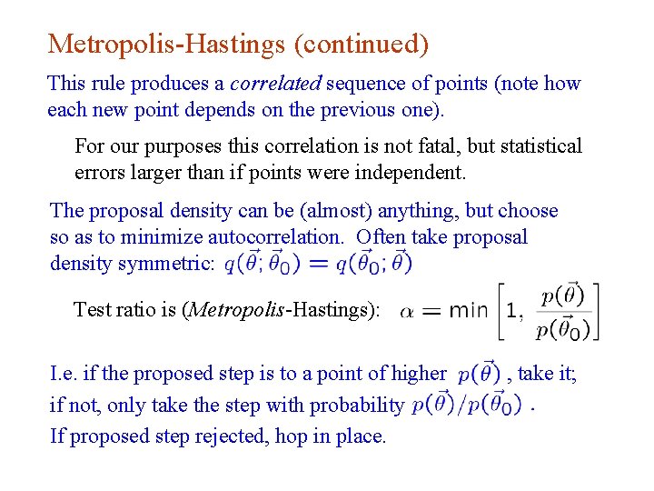
Metropolis-Hastings (continued) This rule produces a correlated sequence of points (note how each new point depends on the previous one). For our purposes this correlation is not fatal, but statistical errors larger than if points were independent. The proposal density can be (almost) anything, but choose so as to minimize autocorrelation. Often take proposal density symmetric: Test ratio is (Metropolis-Hastings): I. e. if the proposed step is to a point of higher if not, only take the step with probability If proposed step rejected, hop in place. G. Cowan Neutrino Summer School / Mainz, 25, 26 May 2018 , take it; 95

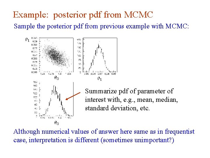
Example: posterior pdf from MCMC Sample the posterior pdf from previous example with MCMC: Summarize pdf of parameter of interest with, e. g. , mean, median, standard deviation, etc. Although numerical values of answer here same as in frequentist case, interpretation is different (sometimes unimportant? ) G. Cowan Neutrino Summer School / Mainz, 25, 26 May 2018 96

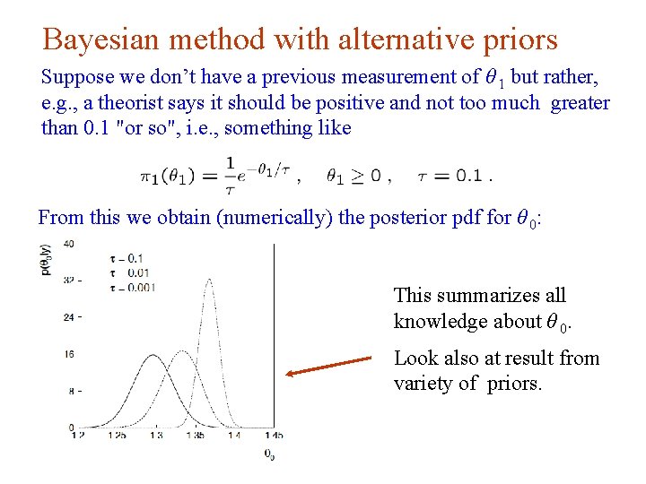
Bayesian method with alternative priors Suppose we don’t have a previous measurement of θ 1 but rather, e. g. , a theorist says it should be positive and not too much greater than 0. 1 "or so", i. e. , something like From this we obtain (numerically) the posterior pdf for θ 0: This summarizes all knowledge about θ 0. Look also at result from variety of priors. G. Cowan Neutrino Summer School / Mainz, 25, 26 May 2018 97

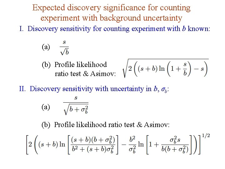
Expected discovery significance for counting experiment with background uncertainty I. Discovery sensitivity for counting experiment with b known: (a) (b) Profile likelihood ratio test & Asimov: II. Discovery sensitivity with uncertainty in b, σb: (a) (b) Profile likelihood ratio test & Asimov: G. Cowan Neutrino Summer School / Mainz, 25, 26 May 2018 98

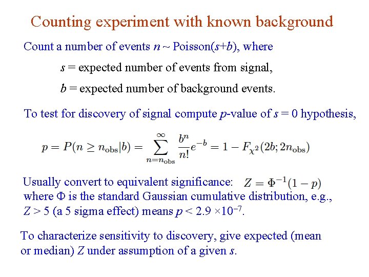
Counting experiment with known background Count a number of events n ~ Poisson(s+b), where s = expected number of events from signal, b = expected number of background events. To test for discovery of signal compute p-value of s = 0 hypothesis, Usually convert to equivalent significance: where Φ is the standard Gaussian cumulative distribution, e. g. , Z > 5 (a 5 sigma effect) means p < 2. 9 × 10 -7. To characterize sensitivity to discovery, give expected (mean or median) Z under assumption of a given s. G. Cowan Neutrino Summer School / Mainz, 25, 26 May 2018 99

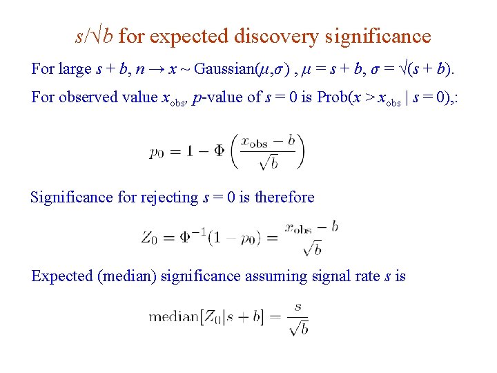
s/√b for expected discovery significance For large s + b, n → x ~ Gaussian(μ, σ ) , μ = s + b, σ = √(s + b). For observed value xobs, p-value of s = 0 is Prob(x > xobs | s = 0), : Significance for rejecting s = 0 is therefore Expected (median) significance assuming signal rate s is G. Cowan Neutrino Summer School / Mainz, 25, 26 May 2018 100

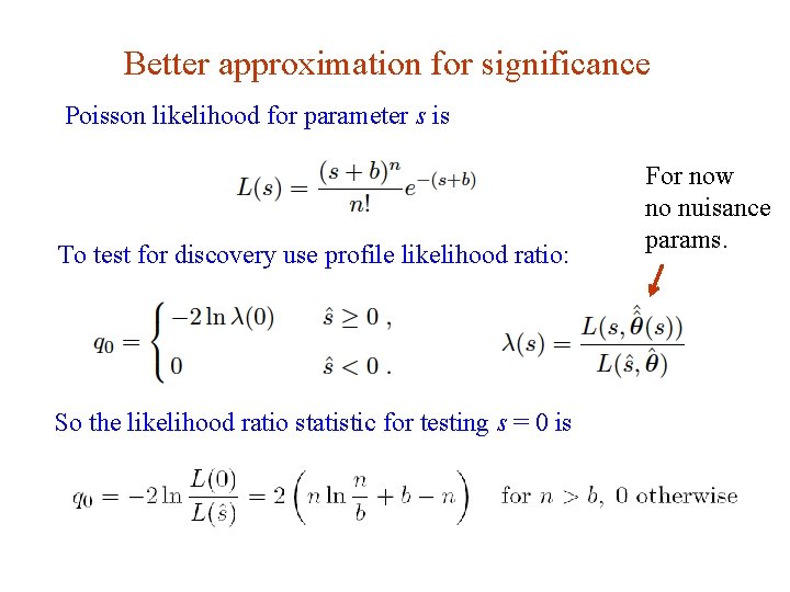
Better approximation for significance Poisson likelihood for parameter s is To test for discovery use profile likelihood ratio: For now no nuisance params. So the likelihood ratio statistic for testing s = 0 is G. Cowan Neutrino Summer School / Mainz, 25, 26 May 2018 101

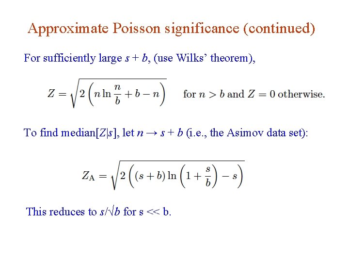
Approximate Poisson significance (continued) For sufficiently large s + b, (use Wilks’ theorem), To find median[Z|s], let n → s + b (i. e. , the Asimov data set): This reduces to s/√b for s << b. G. Cowan Neutrino Summer School / Mainz, 25, 26 May 2018 102

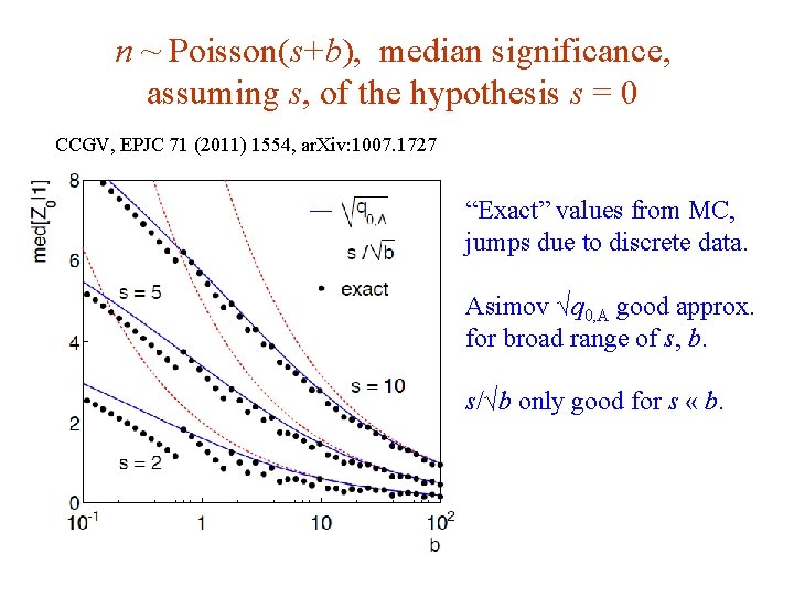
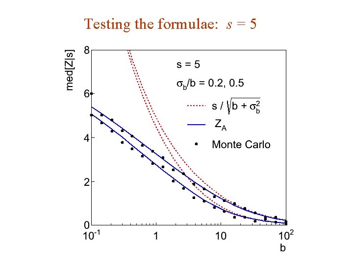
n ~ Poisson(s+b), median significance, assuming s, of the hypothesis s = 0 CCGV, EPJC 71 (2011) 1554, ar. Xiv: 1007. 1727 “Exact” values from MC, jumps due to discrete data. Asimov √q 0, A good approx. for broad range of s, b. s/√b only good for s « b. G. Cowan Neutrino Summer School / Mainz, 25, 26 May 2018 103

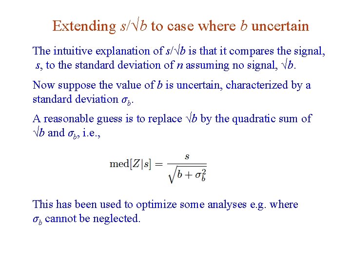
Extending s/√b to case where b uncertain The intuitive explanation of s/√b is that it compares the signal, s, to the standard deviation of n assuming no signal, √b. Now suppose the value of b is uncertain, characterized by a standard deviation σb. A reasonable guess is to replace √b by the quadratic sum of √b and σb, i. e. , This has been used to optimize some analyses e. g. where σb cannot be neglected. G. Cowan Neutrino Summer School / Mainz, 25, 26 May 2018 104

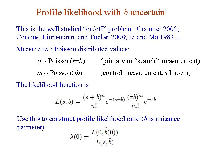
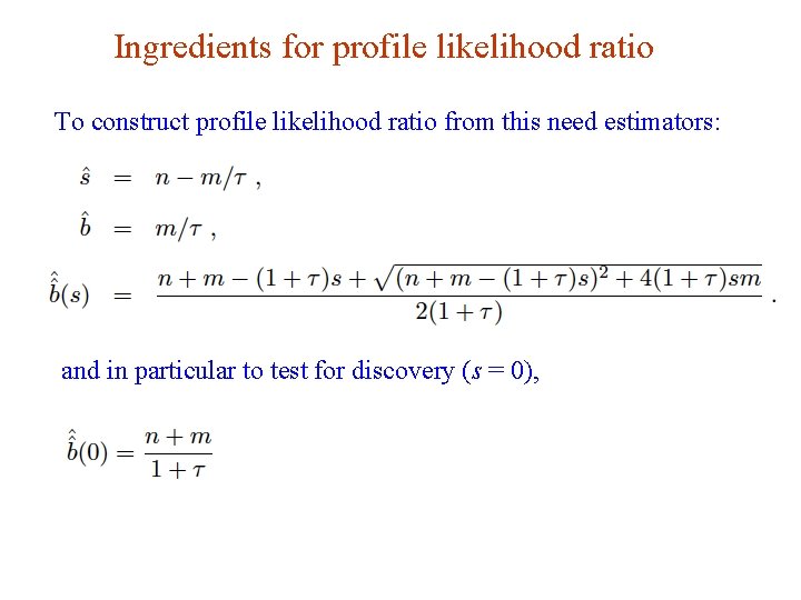
Profile likelihood with b uncertain This is the well studied “on/off” problem: Cranmer 2005; Cousins, Linnemann, and Tucker 2008; Li and Ma 1983, . . . Measure two Poisson distributed values: n ~ Poisson(s+b) (primary or “search” measurement) m ~ Poisson(τb) (control measurement, τ known) The likelihood function is Use this to construct profile likelihood ratio (b is nuisance parmeter): G. Cowan Neutrino Summer School / Mainz, 25, 26 May 2018 105

Ingredients for profile likelihood ratio To construct profile likelihood ratio from this need estimators: and in particular to test for discovery (s = 0), G. Cowan Neutrino Summer School / Mainz, 25, 26 May 2018 106

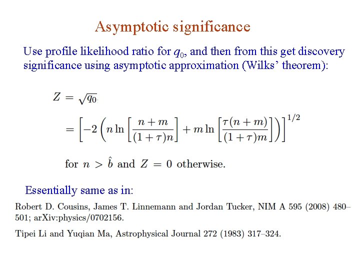
Asymptotic significance Use profile likelihood ratio for q 0, and then from this get discovery significance using asymptotic approximation (Wilks’ theorem): Essentially same as in: G. Cowan Neutrino Summer School / Mainz, 25, 26 May 2018 107

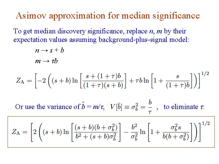
Asimov approximation for median significance To get median discovery significance, replace n, m by their expectation values assuming background-plus-signal model: n→s+b m → τb Or use the variance of ˆb = m/τ, G. Cowan , to eliminate τ: Neutrino Summer School / Mainz, 25, 26 May 2018 108

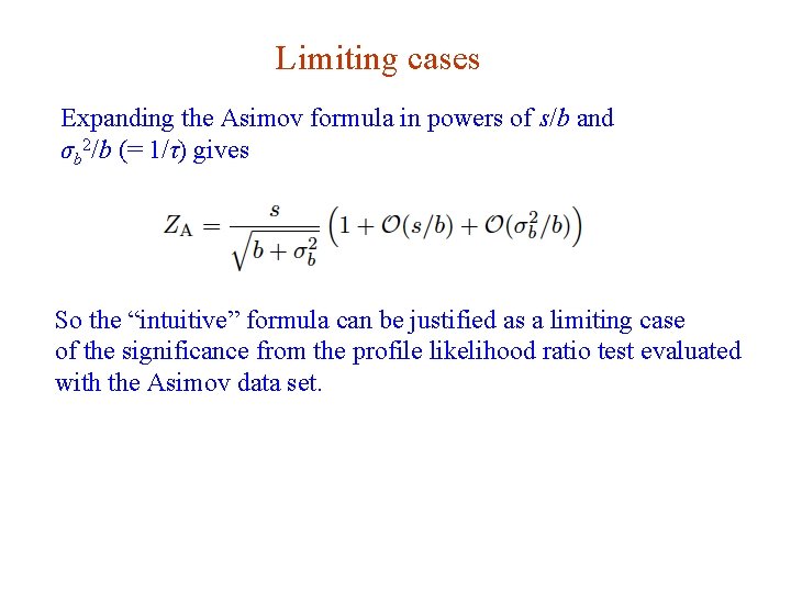
Limiting cases Expanding the Asimov formula in powers of s/b and σb 2/b (= 1/τ) gives So the “intuitive” formula can be justified as a limiting case of the significance from the profile likelihood ratio test evaluated with the Asimov data set. G. Cowan Neutrino Summer School / Mainz, 25, 26 May 2018 109

Testing the formulae: s = 5 G. Cowan Neutrino Summer School / Mainz, 25, 26 May 2018 110

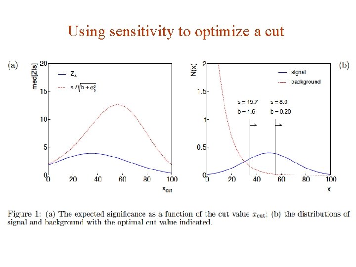
Using sensitivity to optimize a cut G. Cowan Neutrino Summer School / Mainz, 25, 26 May 2018 111

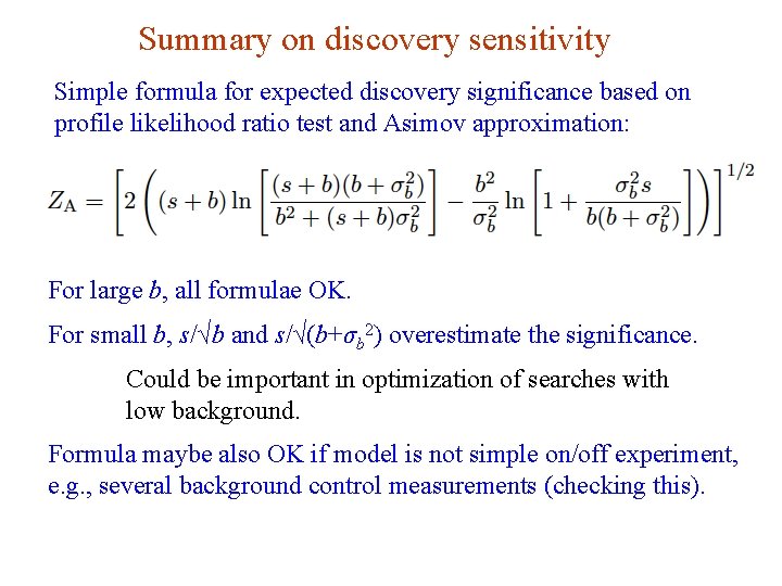
Summary on discovery sensitivity Simple formula for expected discovery significance based on profile likelihood ratio test and Asimov approximation: For large b, all formulae OK. For small b, s/√b and s/√(b+σb 2) overestimate the significance. Could be important in optimization of searches with low background. Formula maybe also OK if model is not simple on/off experiment, e. g. , several background control measurements (checking this). G. Cowan Neutrino Summer School / Mainz, 25, 26 May 2018 112

Finally Three lectures only enough for a brief introduction to: Statistical tests for discovery and limits Multivariate methods Bayesian parameter estimation, MCMC Experimental sensitivity No time for many important topics Properties of estimators (bias, variance) Bayesian approach to discovery (Bayes factors) The look-elsewhere effect, etc. Final thought: once the basic formalism is understood, most of the work focuses on writing down the likelihood, e. g. , P(x|q), and including in it enough parameters to adequately describe the data (true for both Bayesian and frequentist approaches). G. Cowan Neutrino Summer School / Mainz, 25, 26 May 2018 113

Extra slides G. Cowan Neutrino Summer School / Mainz, 25, 26 May 2018 114

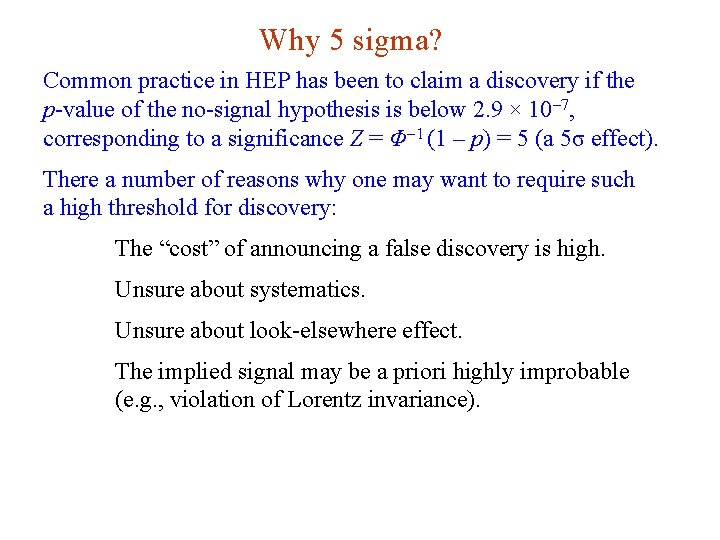
Why 5 sigma? Common practice in HEP has been to claim a discovery if the p-value of the no-signal hypothesis is below 2. 9 × 10 -7, corresponding to a significance Z = Φ-1 (1 – p) = 5 (a 5σ effect). There a number of reasons why one may want to require such a high threshold for discovery: The “cost” of announcing a false discovery is high. Unsure about systematics. Unsure about look-elsewhere effect. The implied signal may be a priori highly improbable (e. g. , violation of Lorentz invariance). G. Cowan Neutrino Summer School / Mainz, 25, 26 May 2018 115

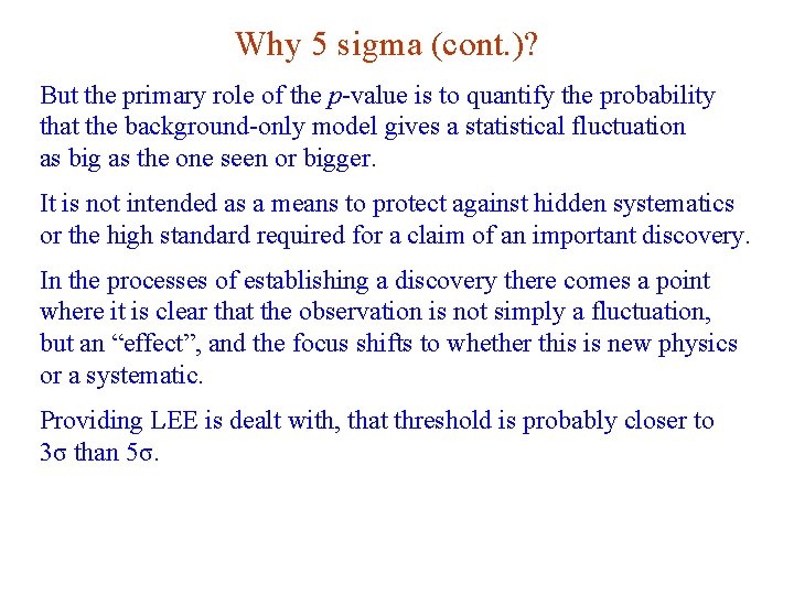
Why 5 sigma (cont. )? But the primary role of the p-value is to quantify the probability that the background-only model gives a statistical fluctuation as big as the one seen or bigger. It is not intended as a means to protect against hidden systematics or the high standard required for a claim of an important discovery. In the processes of establishing a discovery there comes a point where it is clear that the observation is not simply a fluctuation, but an “effect”, and the focus shifts to whether this is new physics or a systematic. Providing LEE is dealt with, that threshold is probably closer to 3σ than 5σ. G. Cowan Neutrino Summer School / Mainz, 25, 26 May 2018 116

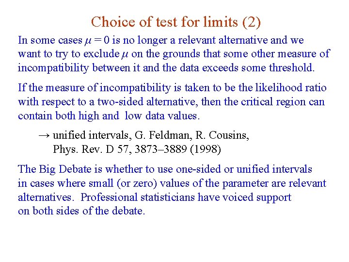
Choice of test for limits (2) In some cases μ = 0 is no longer a relevant alternative and we want to try to exclude μ on the grounds that some other measure of incompatibility between it and the data exceeds some threshold. If the measure of incompatibility is taken to be the likelihood ratio with respect to a two-sided alternative, then the critical region can contain both high and low data values. → unified intervals, G. Feldman, R. Cousins, Phys. Rev. D 57, 3873– 3889 (1998) The Big Debate is whether to use one-sided or unified intervals in cases where small (or zero) values of the parameter are relevant alternatives. Professional statisticians have voiced support on both sides of the debate. G. Cowan Neutrino Summer School / Mainz, 25, 26 May 2018 117

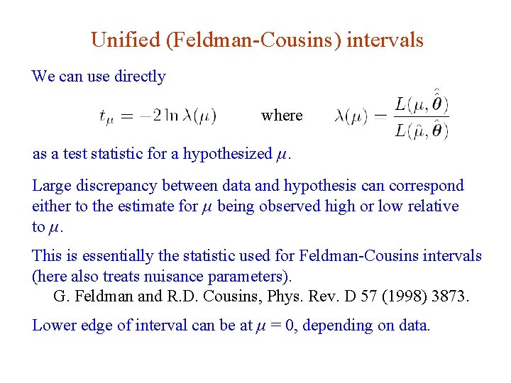
Unified (Feldman-Cousins) intervals We can use directly where as a test statistic for a hypothesized μ. Large discrepancy between data and hypothesis can correspond either to the estimate for μ being observed high or low relative to μ. This is essentially the statistic used for Feldman-Cousins intervals (here also treats nuisance parameters). G. Feldman and R. D. Cousins, Phys. Rev. D 57 (1998) 3873. Lower edge of interval can be at μ = 0, depending on data. G. Cowan Neutrino Summer School / Mainz, 25, 26 May 2018 118

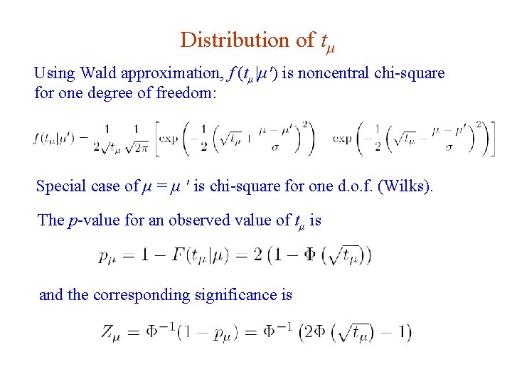
Distribution of tμ Using Wald approximation, f (tμ |μ′) is noncentral chi-square for one degree of freedom: Special case of μ = μ ′ is chi-square for one d. o. f. (Wilks). The p-value for an observed value of tμ is and the corresponding significance is G. Cowan Neutrino Summer School / Mainz, 25, 26 May 2018 119

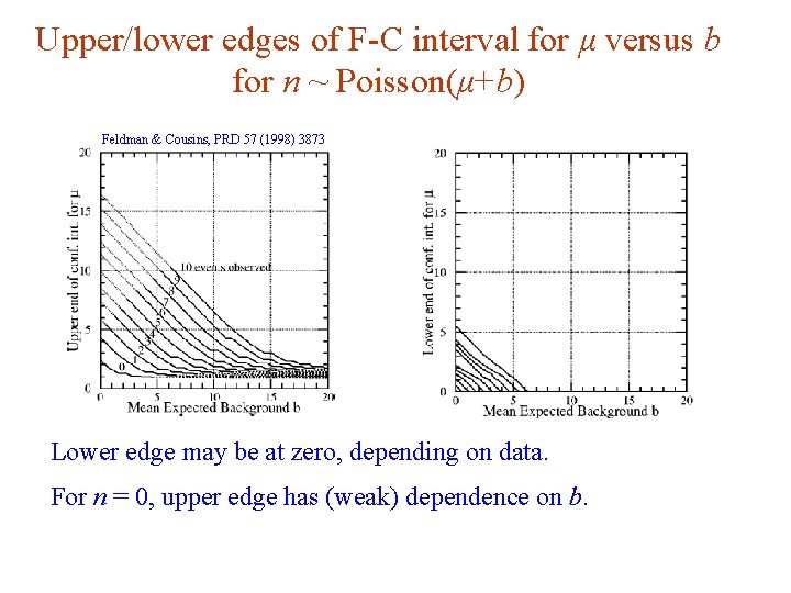
Upper/lower edges of F-C interval for μ versus b for n ~ Poisson(μ+b) Feldman & Cousins, PRD 57 (1998) 3873 Lower edge may be at zero, depending on data. For n = 0, upper edge has (weak) dependence on b. G. Cowan Neutrino Summer School / Mainz, 25, 26 May 2018 120

Feldman-Cousins discussion The initial motivation for Feldman-Cousins (unified) confidence intervals was to eliminate null intervals. The F-C limits are based on a likelihood ratio for a test of μ with respect to the alternative consisting of all other allowed values of μ (not just, say, lower values). The interval’s upper edge is higher than the limit from the onesided test, and lower values of μ may be excluded as well. A substantial downward fluctuation in the data gives a low (but nonzero) limit. This means that when a value of μ is excluded, it is because there is a probability α for the data to fluctuate either high or low in a manner corresponding to less compatibility as measured by the likelihood ratio. G. Cowan Neutrino Summer School / Mainz, 25, 26 May 2018 121

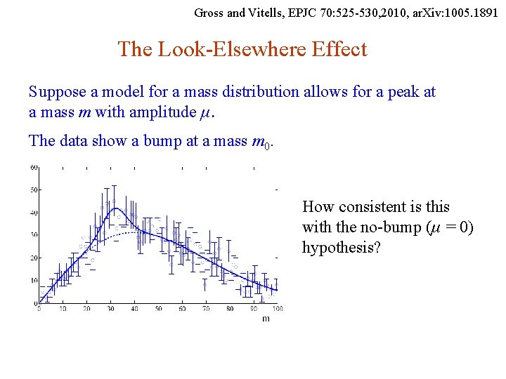
Gross and Vitells, EPJC 70: 525 -530, 2010, ar. Xiv: 1005. 1891 The Look-Elsewhere Effect Suppose a model for a mass distribution allows for a peak at a mass m with amplitude μ. The data show a bump at a mass m 0. How consistent is this with the no-bump (μ = 0) hypothesis? G. Cowan Neutrino Summer School / Mainz, 25, 26 May 2018 122

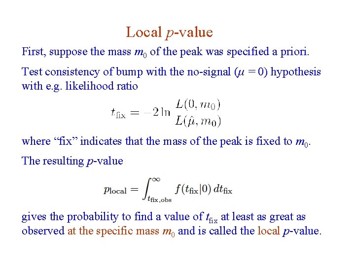
Local p-value First, suppose the mass m 0 of the peak was specified a priori. Test consistency of bump with the no-signal (μ = 0) hypothesis with e. g. likelihood ratio where “fix” indicates that the mass of the peak is fixed to m 0. The resulting p-value gives the probability to find a value of tfix at least as great as observed at the specific mass m 0 and is called the local p-value. G. Cowan Neutrino Summer School / Mainz, 25, 26 May 2018 123

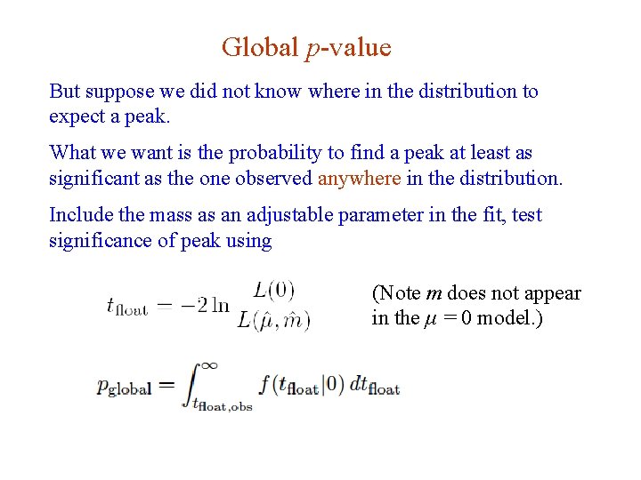
Global p-value But suppose we did not know where in the distribution to expect a peak. What we want is the probability to find a peak at least as significant as the one observed anywhere in the distribution. Include the mass as an adjustable parameter in the fit, test significance of peak using (Note m does not appear in the μ = 0 model. ) G. Cowan Neutrino Summer School / Mainz, 25, 26 May 2018 124

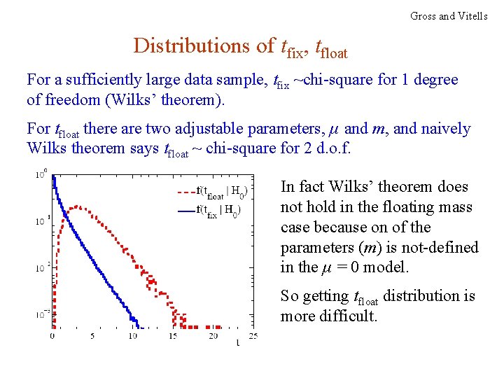
Gross and Vitells Distributions of tfix, tfloat For a sufficiently large data sample, tfix ~chi-square for 1 degree of freedom (Wilks’ theorem). For tfloat there are two adjustable parameters, μ and m, and naively Wilks theorem says tfloat ~ chi-square for 2 d. o. f. In fact Wilks’ theorem does not hold in the floating mass case because on of the parameters (m) is not-defined in the μ = 0 model. So getting tfloat distribution is more difficult. G. Cowan Neutrino Summer School / Mainz, 25, 26 May 2018 125

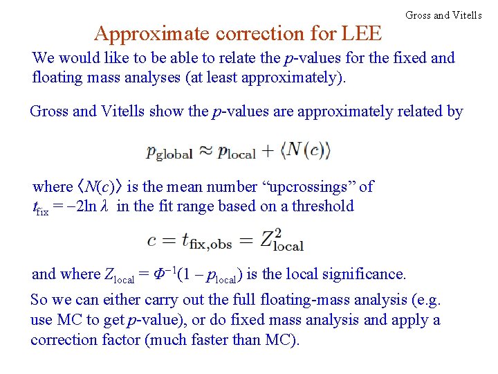
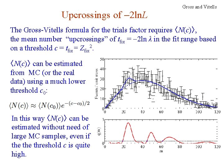
Approximate correction for LEE Gross and Vitells We would like to be able to relate the p-values for the fixed and floating mass analyses (at least approximately). Gross and Vitells show the p-values are approximately related by where 〈N(c)〉 is the mean number “upcrossings” of tfix = -2 ln λ in the fit range based on a threshold and where Zlocal = Φ-1(1 – plocal) is the local significance. So we can either carry out the full floating-mass analysis (e. g. use MC to get p-value), or do fixed mass analysis and apply a correction factor (much faster than MC). G. Cowan Neutrino Summer School / Mainz, 25, 26 May 2018 126

Upcrossings of -2 ln. L Gross and Vitells The Gross-Vitells formula for the trials factor requires 〈N(c)〉, the mean number “upcrossings” of tfix = -2 ln λ in the fit range based on a threshold c = tfix= Zfix 2. 〈N(c)〉 can be estimated from MC (or the real data) using a much lower threshold c 0: In this way 〈N(c)〉 can be estimated without need of large MC samples, even if the threshold c is quite high. G. Cowan Neutrino Summer School / Mainz, 25, 26 May 2018 127

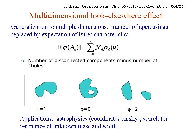
Vitells and Gross, Astropart. Phys. 35 (2011) 230 -234; ar. Xiv: 1105. 4355 Multidimensional look-elsewhere effect Generalization to multiple dimensions: number of upcrossings replaced by expectation of Euler characteristic: Applications: astrophysics (coordinates on sky), search for resonance of unknown mass and width, . . . G. Cowan Neutrino Summer School / Mainz, 25, 26 May 2018 128

Summary on Look-Elsewhere Effect Remember the Look-Elsewhere Effect is when we test a single model (e. g. , SM) with multiple observations, i. . e, in mulitple places. Note there is no look-elsewhere effect when considering exclusion limits. There we test specific signal models (typically once) and say whether each is excluded. With exclusion there is, however, the also problematic issue of testing many signal models (or parameter values) and thus excluding some for which one has little or no sensitivity. Approximate correction for LEE should be sufficient, and one should also report the uncorrected significance. “There's no sense in being precise when you don't even know what you're talking about. ” –– John von Neumann G. Cowan Neutrino Summer School / Mainz, 25, 26 May 2018 129