Statistical Methods for Particle Physics Day 2 Statistical

Statistical Methods for Particle Physics Day 2: Statistical Tests and Limits https: //indico. desy. de/indico/event/19085/ Terascale Statistics School DESY, 19 -23 February, 2018 Glen Cowan Physics Department Royal Holloway, University of London g. cowan@rhul. ac. uk www. pp. rhul. ac. uk/~cowan G. Cowan DESY Terascale School of Statistics / 19 -23 Feb 2018 / Day 2 1

Outline Day 1: Introduction and parameter estimation Probability, random variables, pdfs Parameter estimation maximum likelihood least squares Bayesian parameter estimation Introduction to unfolding Day 2: Discovery and Limits Comments on multivariate methods (brief) p-values Testing the background-only hypothesis: discovery Testing signal hypotheses: setting limits Experimental sensitivity G. Cowan DESY Terascale School of Statistics / 19 -23 Feb 2018 / Day 2 2

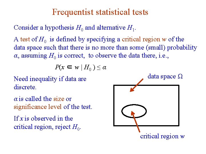
Frequentist statistical tests Consider a hypothesis H 0 and alternative H 1. A test of H 0 is defined by specifying a critical region w of the data space such that there is no more than some (small) probability α, assuming H 0 is correct, to observe the data there, i. e. , P(x ∈ w | H 0 ) ≤ α Need inequality if data are discrete. data space Ω α is called the size or significance level of the test. If x is observed in the critical region, reject H 0. critical region w G. Cowan DESY Terascale School of Statistics / 19 -23 Feb 2018 / Day 2 3

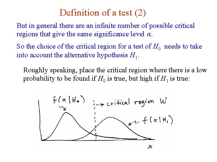
Definition of a test (2) But in general there an infinite number of possible critical regions that give the same significance level α. So the choice of the critical region for a test of H 0 needs to take into account the alternative hypothesis H 1. Roughly speaking, place the critical region where there is a low probability to be found if H 0 is true, but high if H 1 is true: G. Cowan DESY Terascale School of Statistics / 19 -23 Feb 2018 / Day 2 4

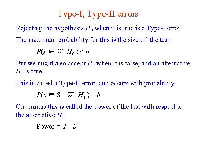
Type-I, Type-II errors Rejecting the hypothesis H 0 when it is true is a Type-I error. The maximum probability for this is the size of the test: P(x ∈ W | H 0 ) ≤ α But we might also accept H 0 when it is false, and an alternative H 1 is true. This is called a Type-II error, and occurs with probability P(x ∈ S - W | H 1 ) = β One minus this is called the power of the test with respect to the alternative H 1: Power = 1 - β G. Cowan DESY Terascale School of Statistics / 19 -23 Feb 2018 / Day 2 5

A simulated SUSY event high p. T jets of hadrons high p. T muons p p missing transverse energy G. Cowan DESY Terascale School of Statistics / 19 -23 Feb 2018 / Day 2 6

Background events This event from Standard Model ttbar production also has high p. T jets and muons, and some missing transverse energy. → can easily mimic a SUSY event. G. Cowan DESY Terascale School of Statistics / 19 -23 Feb 2018 / Day 2 7

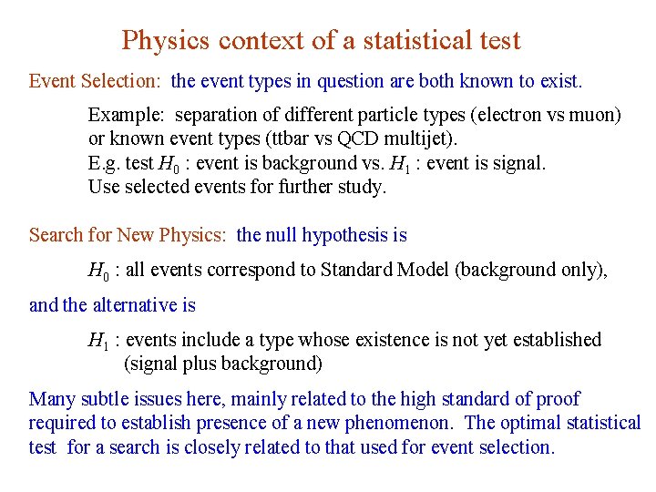
Physics context of a statistical test Event Selection: the event types in question are both known to exist. Example: separation of different particle types (electron vs muon) or known event types (ttbar vs QCD multijet). E. g. test H 0 : event is background vs. H 1 : event is signal. Use selected events for further study. Search for New Physics: the null hypothesis is H 0 : all events correspond to Standard Model (background only), and the alternative is H 1 : events include a type whose existence is not yet established (signal plus background) Many subtle issues here, mainly related to the high standard of proof required to establish presence of a new phenomenon. The optimal statistical test for a search is closely related to that used for event selection. G. Cowan DESY Terascale School of Statistics / 19 -23 Feb 2018 / Day 2 8

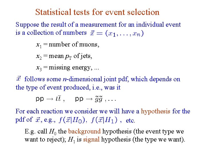
Statistical tests for event selection Suppose the result of a measurement for an individual event is a collection of numbers x 1 = number of muons, x 2 = mean p. T of jets, x 3 = missing energy, . . . follows some n-dimensional joint pdf, which depends on the type of event produced, i. e. , was it For each reaction we consider we will have a hypothesis for the pdf of , e. g. , etc. E. g. call H 0 the background hypothesis (the event type we want to reject); H 1 is signal hypothesis (the type we want). G. Cowan DESY Terascale School of Statistics / 19 -23 Feb 2018 / Day 2 9

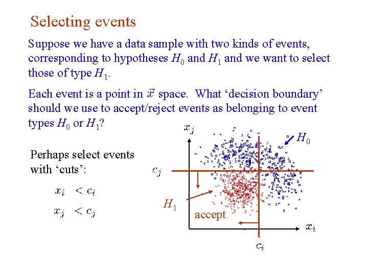
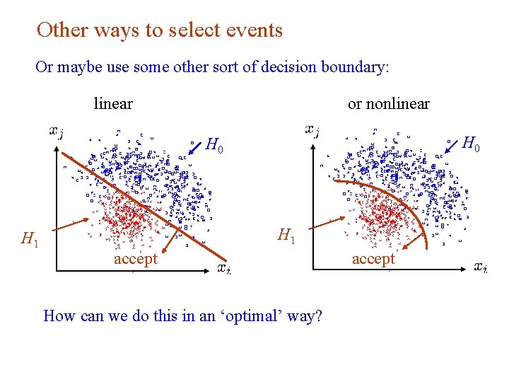
Selecting events Suppose we have a data sample with two kinds of events, corresponding to hypotheses H 0 and H 1 and we want to select those of type H 1. Each event is a point in space. What ‘decision boundary’ should we use to accept/reject events as belonging to event types H 0 or H 1? H 0 Perhaps select events with ‘cuts’: H 1 G. Cowan accept DESY Terascale School of Statistics / 19 -23 Feb 2018 / Day 2 10

Other ways to select events Or maybe use some other sort of decision boundary: linear or nonlinear H 0 H 1 accept How can we do this in an ‘optimal’ way? G. Cowan DESY Terascale School of Statistics / 19 -23 Feb 2018 / Day 2 11

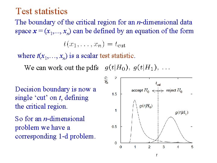
Test statistics The boundary of the critical region for an n-dimensional data space x = (x 1, . . . , xn) can be defined by an equation of the form where t(x 1, …, xn) is a scalar test statistic. We can work out the pdfs Decision boundary is now a single ‘cut’ on t, defining the critical region. So for an n-dimensional problem we have a corresponding 1 -d problem. G. Cowan DESY Terascale School of Statistics / 19 -23 Feb 2018 / Day 2 12

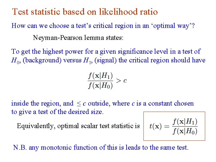
Test statistic based on likelihood ratio How can we choose a test’s critical region in an ‘optimal way’? Neyman-Pearson lemma states: To get the highest power for a given significance level in a test of H 0, (background) versus H 1, (signal) the critical region should have inside the region, and ≤ c outside, where c is a constant chosen to give a test of the desired size. Equivalently, optimal scalar test statistic is N. B. any monotonic function of this is leads to the same test. G. Cowan DESY Terascale School of Statistics / 19 -23 Feb 2018 / Day 2 13

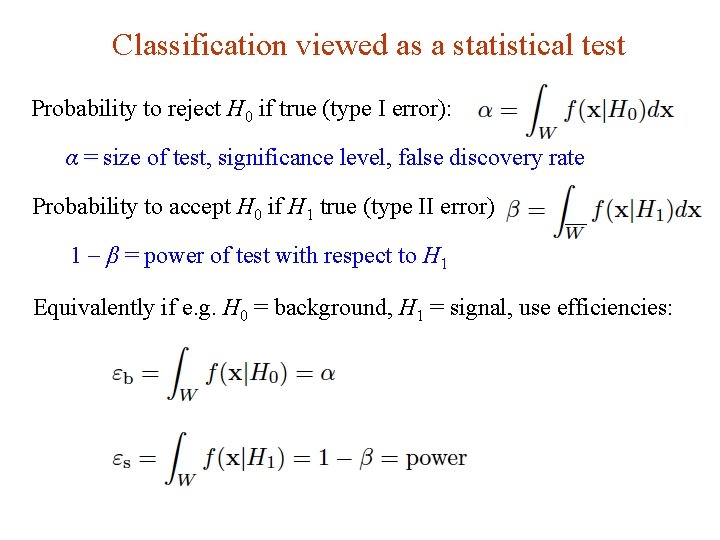
Classification viewed as a statistical test Probability to reject H 0 if true (type I error): α = size of test, significance level, false discovery rate Probability to accept H 0 if H 1 true (type II error): 1 - β = power of test with respect to H 1 Equivalently if e. g. H 0 = background, H 1 = signal, use efficiencies: G. Cowan DESY Terascale School of Statistics / 19 -23 Feb 2018 / Day 2 14

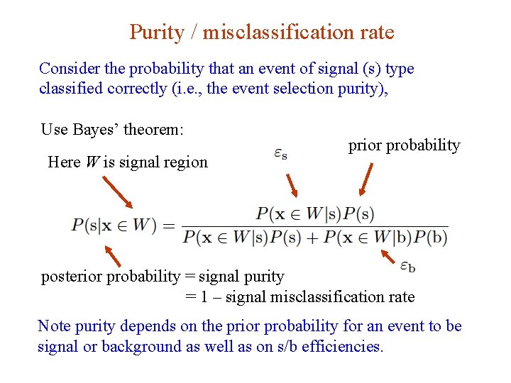
Purity / misclassification rate Consider the probability that an event of signal (s) type classified correctly (i. e. , the event selection purity), Use Bayes’ theorem: Here W is signal region prior probability posterior probability = signal purity = 1 – signal misclassification rate Note purity depends on the prior probability for an event to be signal or background as well as on s/b efficiencies. G. Cowan DESY Terascale School of Statistics / 19 -23 Feb 2018 / Day 2 15

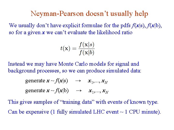
Neyman-Pearson doesn’t usually help We usually don’t have explicit formulae for the pdfs f (x|s), f (x|b), so for a given x we can’t evaluate the likelihood ratio Instead we may have Monte Carlo models for signal and background processes, so we can produce simulated data: generate x ~ f (x|s) → x 1, . . . , x. N generate x ~ f (x|b) → x 1, . . . , x. N This gives samples of “training data” with events of known type. Can be expensive (1 fully simulated LHC event ~ 1 CPU minute). G. Cowan DESY Terascale School of Statistics / 19 -23 Feb 2018 / Day 2 16

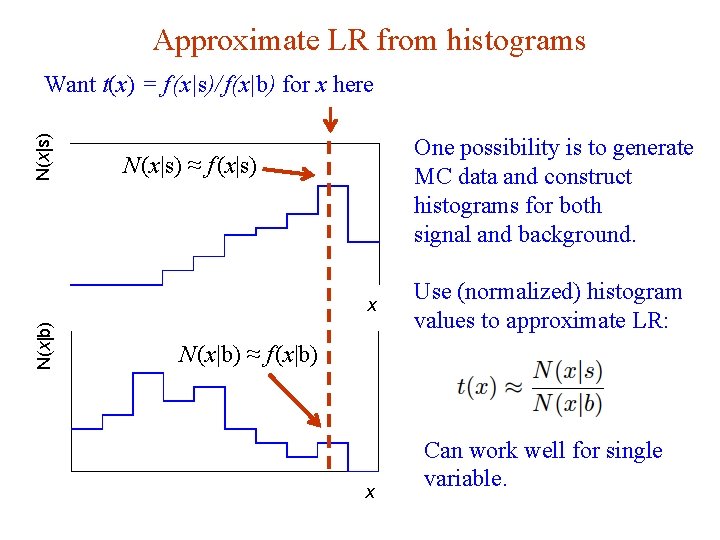
Approximate LR from histograms N(x|s) Want t(x) = f (x|s)/ f(x|b) for x here One possibility is to generate MC data and construct histograms for both signal and background. N (x|s) ≈ f (x|s) N(x|b) x N (x|b) ≈ f (x|b) x G. Cowan Use (normalized) histogram values to approximate LR: Can work well for single variable. DESY Terascale School of Statistics / 19 -23 Feb 2018 / Day 2 17

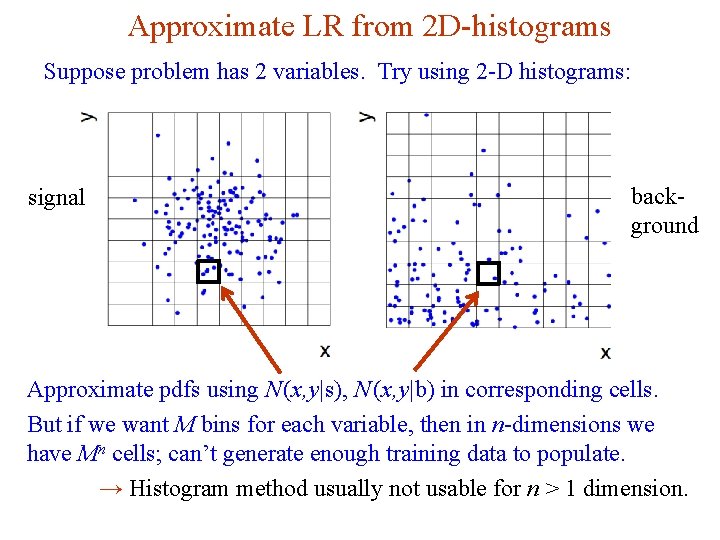
Approximate LR from 2 D-histograms Suppose problem has 2 variables. Try using 2 -D histograms: background signal Approximate pdfs using N (x, y|s), N (x, y|b) in corresponding cells. But if we want M bins for each variable, then in n-dimensions we have Mn cells; can’t generate enough training data to populate. → Histogram method usually not usable for n > 1 dimension. G. Cowan DESY Terascale School of Statistics / 19 -23 Feb 2018 / Day 2 18

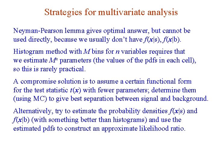
Strategies for multivariate analysis Neyman-Pearson lemma gives optimal answer, but cannot be used directly, because we usually don’t have f (x|s), f (x|b). Histogram method with M bins for n variables requires that we estimate Mn parameters (the values of the pdfs in each cell), so this is rarely practical. A compromise solution is to assume a certain functional form for the test statistic t (x) with fewer parameters; determine them (using MC) to give best separation between signal and background. Alternatively, try to estimate the probability densities f (x|s) and f (x|b) (with something better than histograms) and use the estimated pdfs to construct an approximate likelihood ratio. G. Cowan DESY Terascale School of Statistics / 19 -23 Feb 2018 / Day 2 19

Multivariate methods Many new (and some old) methods: Fisher discriminant (Deep) neural networks Kernel density methods Support Vector Machines Decision trees Boosting Bagging G. Cowan DESY Terascale School of Statistics / 19 -23 Feb 2018 / Day 2 20

Resources on multivariate methods C. M. Bishop, Pattern Recognition and Machine Learning, Springer, 2006 T. Hastie, R. Tibshirani, J. Friedman, The Elements of Statistical Learning, 2 nd ed. , Springer, 2009 R. Duda, P. Hart, D. Stork, Pattern Classification, 2 nd ed. , Wiley, 2001 A. Webb, Statistical Pattern Recognition, 2 nd ed. , Wiley, 2002. Ilya Narsky and Frank C. Porter, Statistical Analysis Techniques in Particle Physics, Wiley, 2014. 朱永生 （�著），��数据多元��分析， 科学出版社， 北 京，2009。 G. Cowan DESY Terascale School of Statistics / 19 -23 Feb 2018 / Day 2 21

Software Rapidly growing area of development – two important resources: TMVA, Höcker, Stelzer, Tegenfeldt, Voss, physics/0703039 From tmva. sourceforge. net, also distributed with ROOT Variety of classifiers Good manual, widely used in HEP scikit-learn Python-based tools for Machine Learning scikit-learn. org Large user community G. Cowan DESY Terascale School of Statistics / 19 -23 Feb 2018 / Day 2 22

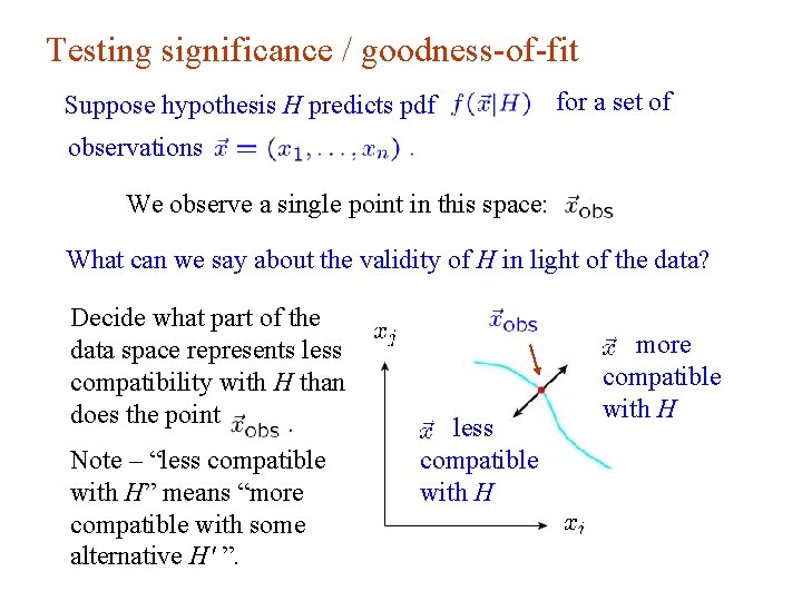
Testing significance / goodness-of-fit Suppose hypothesis H predicts pdf for a set of observations We observe a single point in this space: What can we say about the validity of H in light of the data? Decide what part of the data space represents less compatibility with H than does the point Note – “less compatible with H” means “more compatible with some alternative H′ ”. G. Cowan less compatible with H DESY Terascale School of Statistics / 19 -23 Feb 2018 / Day 2 more compatible with H 23

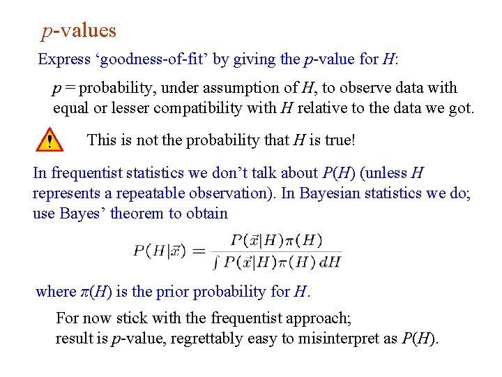
p-values Express ‘goodness-of-fit’ by giving the p-value for H: p = probability, under assumption of H, to observe data with equal or lesser compatibility with H relative to the data we got. This is not the probability that H is true! In frequentist statistics we don’t talk about P(H) (unless H represents a repeatable observation). In Bayesian statistics we do; use Bayes’ theorem to obtain where π(H) is the prior probability for H. For now stick with the frequentist approach; result is p-value, regrettably easy to misinterpret as P(H). G. Cowan DESY Terascale School of Statistics / 19 -23 Feb 2018 / Day 2 24

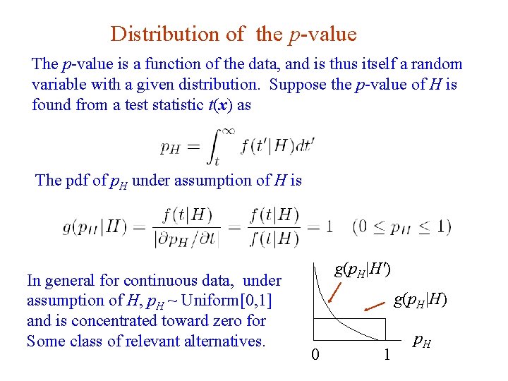
Distribution of the p-value The p-value is a function of the data, and is thus itself a random variable with a given distribution. Suppose the p-value of H is found from a test statistic t(x) as The pdf of p. H under assumption of H is In general for continuous data, under assumption of H, p. H ~ Uniform[0, 1] and is concentrated toward zero for Some class of relevant alternatives. G. Cowan g(p. H|H′) g(p. H|H) 0 DESY Terascale School of Statistics / 19 -23 Feb 2018 / Day 2 1 p. H 25

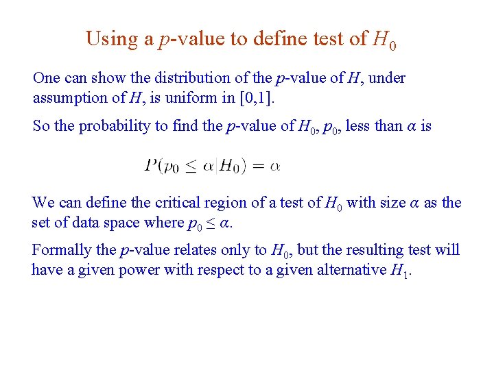
Using a p-value to define test of H 0 One can show the distribution of the p-value of H, under assumption of H, is uniform in [0, 1]. So the probability to find the p-value of H 0, p 0, less than α is We can define the critical region of a test of H 0 with size α as the set of data space where p 0 ≤ α. Formally the p-value relates only to H 0, but the resulting test will have a given power with respect to a given alternative H 1. G. Cowan DESY Terascale School of Statistics / 19 -23 Feb 2018 / Day 2 26

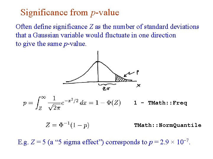
Significance from p-value Often define significance Z as the number of standard deviations that a Gaussian variable would fluctuate in one direction to give the same p-value. 1 - TMath: : Freq TMath: : Norm. Quantile E. g. Z = 5 (a “ 5 sigma effect”) corresponds to p = 2. 9 × 10 -7. G. Cowan DESY Terascale School of Statistics / 19 -23 Feb 2018 / Day 2 27

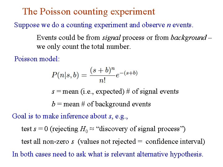
The Poisson counting experiment Suppose we do a counting experiment and observe n events. Events could be from signal process or from background – we only count the total number. Poisson model: s = mean (i. e. , expected) # of signal events b = mean # of background events Goal is to make inference about s, e. g. , test s = 0 (rejecting H 0 ≈ “discovery of signal process”) test all non-zero s (values not rejected = confidence interval) In both cases need to ask what is relevant alternative hypothesis. G. Cowan DESY Terascale School of Statistics / 19 -23 Feb 2018 / Day 2 28

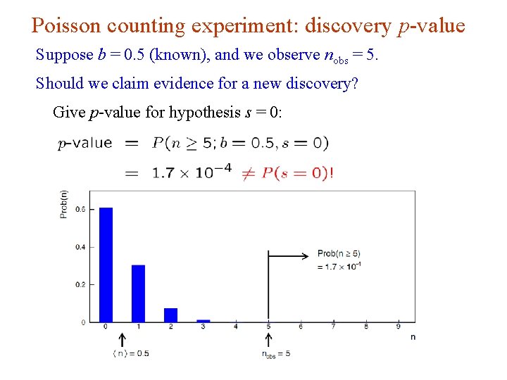
Poisson counting experiment: discovery p-value Suppose b = 0. 5 (known), and we observe nobs = 5. Should we claim evidence for a new discovery? Give p-value for hypothesis s = 0: G. Cowan DESY Terascale School of Statistics / 19 -23 Feb 2018 / Day 2 29

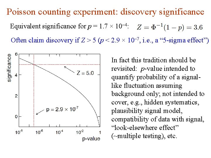
Poisson counting experiment: discovery significance Equivalent significance for p = 1. 7 × 10 -4: Often claim discovery if Z > 5 (p < 2. 9 × 10 -7, i. e. , a “ 5 -sigma effect”) In fact this tradition should be revisited: p-value intended to quantify probability of a signallike fluctuation assuming background only; not intended to cover, e. g. , hidden systematics, plausibility signal model, compatibility of data with signal, “look-elsewhere effect” (~multiple testing), etc. G. Cowan DESY Terascale School of Statistics / 19 -23 Feb 2018 / Day 2 30

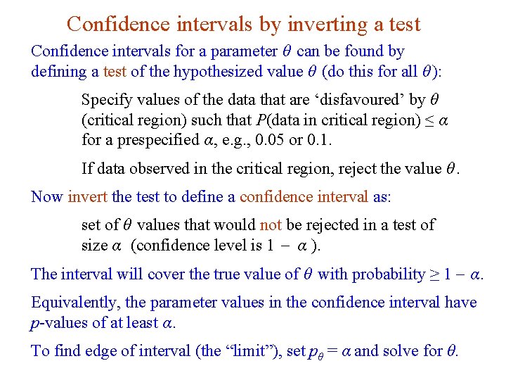
Confidence intervals by inverting a test Confidence intervals for a parameter θ can be found by defining a test of the hypothesized value θ (do this for all θ ): Specify values of the data that are ‘disfavoured’ by θ (critical region) such that P(data in critical region) ≤ α for a prespecified α, e. g. , 0. 05 or 0. 1. If data observed in the critical region, reject the value θ. Now invert the test to define a confidence interval as: set of θ values that would not be rejected in a test of size α (confidence level is 1 - α ). The interval will cover the true value of θ with probability ≥ 1 - α. Equivalently, the parameter values in the confidence interval have p-values of at least α. To find edge of interval (the “limit”), set pθ = α and solve for θ. G. Cowan DESY Terascale School of Statistics / 19 -23 Feb 2018 / Day 2 31

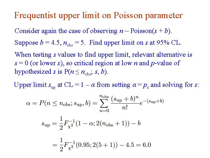
Frequentist upper limit on Poisson parameter Consider again the case of observing n ~ Poisson(s + b). Suppose b = 4. 5, nobs = 5. Find upper limit on s at 95% CL. When testing s values to find upper limit, relevant alternative is s = 0 (or lower s), so critical region at low n and p-value of hypothesized s is P(n ≤ nobs; s, b). Upper limit sup at CL = 1 – α from setting α = ps and solving for s: G. Cowan DESY Terascale School of Statistics / 19 -23 Feb 2018 / Day 2 32

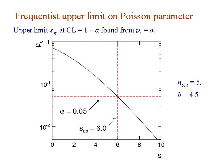
Frequentist upper limit on Poisson parameter Upper limit sup at CL = 1 – α found from ps = α. nobs = 5, b = 4. 5 G. Cowan DESY Terascale School of Statistics / 19 -23 Feb 2018 / Day 2 33

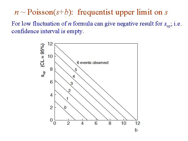
n ~ Poisson(s+b): frequentist upper limit on s For low fluctuation of n formula can give negative result for sup; i. e. confidence interval is empty. G. Cowan DESY Terascale School of Statistics / 19 -23 Feb 2018 / Day 2 34

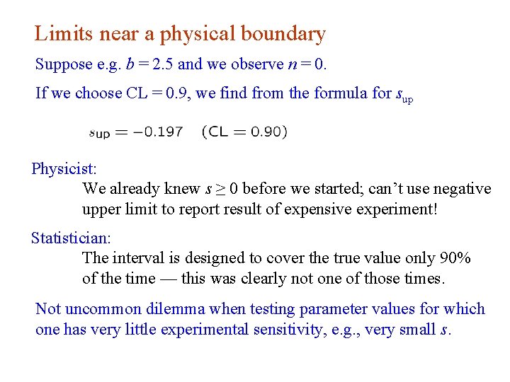
Limits near a physical boundary Suppose e. g. b = 2. 5 and we observe n = 0. If we choose CL = 0. 9, we find from the formula for sup Physicist: We already knew s ≥ 0 before we started; can’t use negative upper limit to report result of expensive experiment! Statistician: The interval is designed to cover the true value only 90% of the time — this was clearly not one of those times. Not uncommon dilemma when testing parameter values for which one has very little experimental sensitivity, e. g. , very small s. G. Cowan DESY Terascale School of Statistics / 19 -23 Feb 2018 / Day 2 35

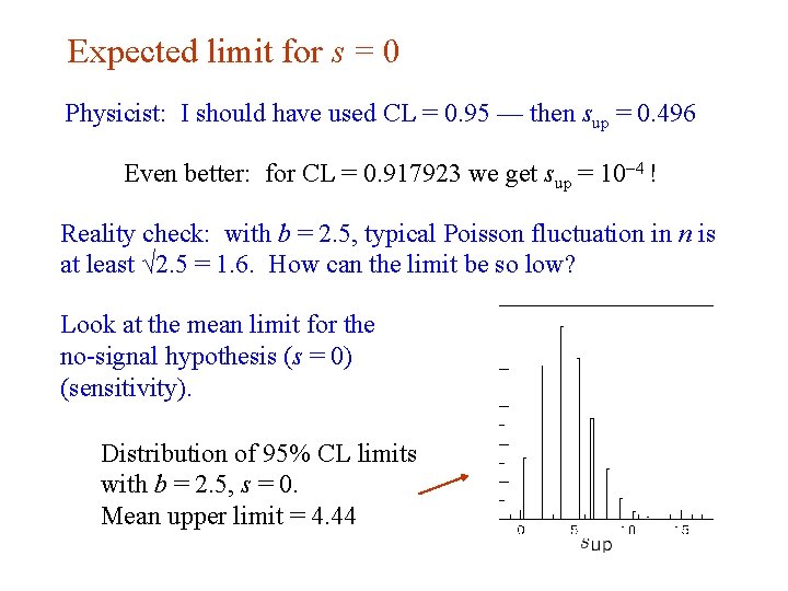
Expected limit for s = 0 Physicist: I should have used CL = 0. 95 — then sup = 0. 496 Even better: for CL = 0. 917923 we get sup = 10 -4 ! Reality check: with b = 2. 5, typical Poisson fluctuation in n is at least √ 2. 5 = 1. 6. How can the limit be so low? Look at the mean limit for the no-signal hypothesis (s = 0) (sensitivity). Distribution of 95% CL limits with b = 2. 5, s = 0. Mean upper limit = 4. 44 G. Cowan DESY Terascale School of Statistics / 19 -23 Feb 2018 / Day 2 36

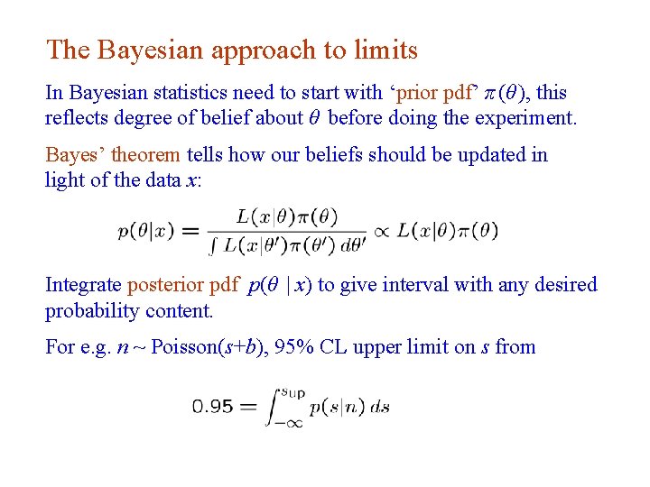
The Bayesian approach to limits In Bayesian statistics need to start with ‘prior pdf’ π (θ ), this reflects degree of belief about θ before doing the experiment. Bayes’ theorem tells how our beliefs should be updated in light of the data x: Integrate posterior pdf p(θ | x) to give interval with any desired probability content. For e. g. n ~ Poisson(s+b), 95% CL upper limit on s from G. Cowan DESY Terascale School of Statistics / 19 -23 Feb 2018 / Day 2 37

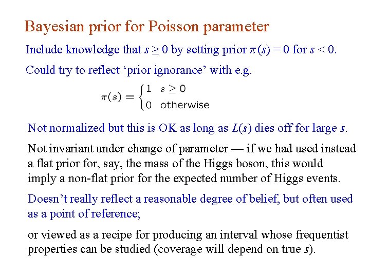
Bayesian prior for Poisson parameter Include knowledge that s ≥ 0 by setting prior π (s) = 0 for s < 0. Could try to reflect ‘prior ignorance’ with e. g. Not normalized but this is OK as long as L(s) dies off for large s. Not invariant under change of parameter — if we had used instead a flat prior for, say, the mass of the Higgs boson, this would imply a non-flat prior for the expected number of Higgs events. Doesn’t really reflect a reasonable degree of belief, but often used as a point of reference; or viewed as a recipe for producing an interval whose frequentist properties can be studied (coverage will depend on true s). G. Cowan DESY Terascale School of Statistics / 19 -23 Feb 2018 / Day 2 38

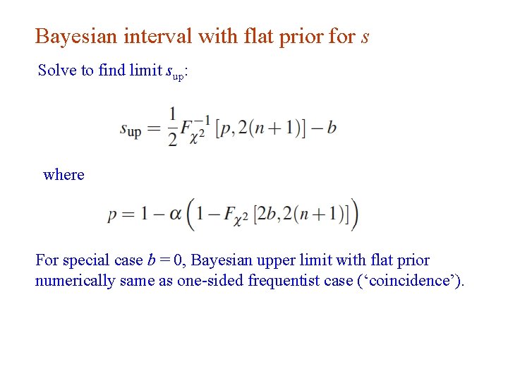
Bayesian interval with flat prior for s Solve to find limit sup: where For special case b = 0, Bayesian upper limit with flat prior numerically same as one-sided frequentist case (‘coincidence’). G. Cowan DESY Terascale School of Statistics / 19 -23 Feb 2018 / Day 2 39

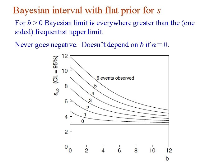
Bayesian interval with flat prior for s For b > 0 Bayesian limit is everywhere greater than the (one sided) frequentist upper limit. Never goes negative. Doesn’t depend on b if n = 0. G. Cowan DESY Terascale School of Statistics / 19 -23 Feb 2018 / Day 2 40

Priors from formal rules Because of difficulties in encoding a vague degree of belief in a prior, one often attempts to derive the prior from formal rules, e. g. , to satisfy certain invariance principles or to provide maximum information gain for a certain set of measurements. Often called “objective priors” Form basis of Objective Bayesian Statistics The priors do not reflect a degree of belief (but might represent possible extreme cases). In Objective Bayesian analysis, can use the intervals in a frequentist way, i. e. , regard Bayes’ theorem as a recipe to produce an interval with certain coverage properties. G. Cowan DESY Terascale School of Statistics / 19 -23 Feb 2018 / Day 2 41

Priors from formal rules (cont. ) For a review of priors obtained by formal rules see, e. g. , Formal priors have not been widely used in HEP, but there is recent interest in this direction, especially the reference priors of Bernardo and Berger; see e. g. L. Demortier, S. Jain and H. Prosper, Reference priors for high energy physics, Phys. Rev. D 82 (2010) 034002, ar. Xiv: 1002. 1111. D. Casadei, Reference analysis of the signal + background model in counting experiments, JINST 7 (2012) 01012; ar. Xiv: 1108. 4270. G. Cowan DESY Terascale School of Statistics / 19 -23 Feb 2018 / Day 2 42

Approximate confidence intervals/regions from the likelihood function Suppose we test parameter value(s) θ = (θ 1, . . . , θn) using the ratio Lower λ(θ) means worse agreement between data and hypothesized θ. Equivalently, usually define so higher tθ means worse agreement between θ and the data. p-value of θ therefore G. Cowan DESY Terascale School of Statistics / 19 -23 Feb 2018 / Day 2 need pdf 43

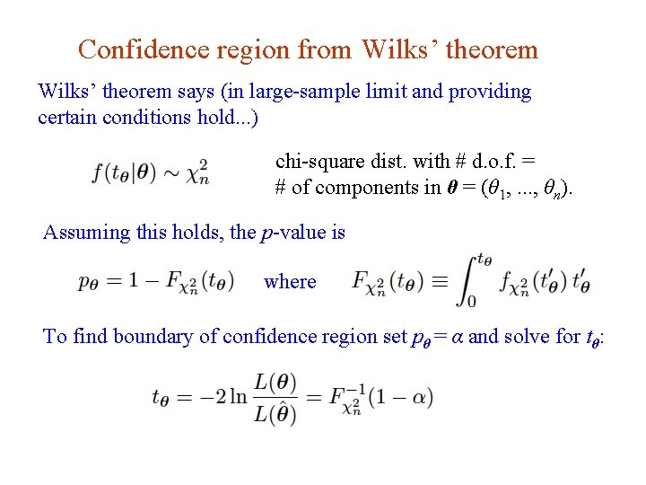
Confidence region from Wilks’ theorem says (in large-sample limit and providing certain conditions hold. . . ) chi-square dist. with # d. o. f. = # of components in θ = (θ 1, . . . , θn). Assuming this holds, the p-value is where To find boundary of confidence region set pθ = α and solve for tθ: G. Cowan DESY Terascale School of Statistics / 19 -23 Feb 2018 / Day 2 44

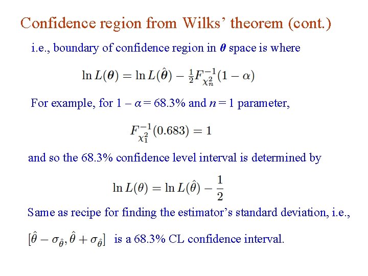
Confidence region from Wilks’ theorem (cont. ) i. e. , boundary of confidence region in θ space is where For example, for 1 – α = 68. 3% and n = 1 parameter, and so the 68. 3% confidence level interval is determined by Same as recipe for finding the estimator’s standard deviation, i. e. , is a 68. 3% CL confidence interval. G. Cowan DESY Terascale School of Statistics / 19 -23 Feb 2018 / Day 2 45

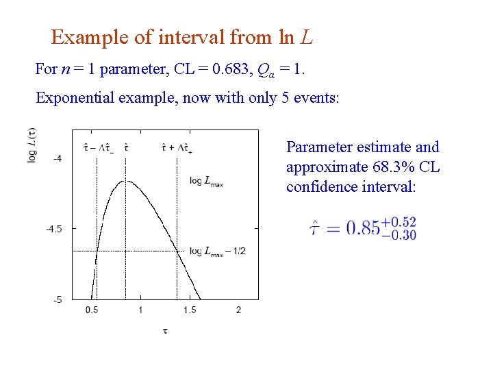
Example of interval from ln L For n = 1 parameter, CL = 0. 683, Qα = 1. Exponential example, now with only 5 events: Parameter estimate and approximate 68. 3% CL confidence interval: G. Cowan DESY Terascale School of Statistics / 19 -23 Feb 2018 / Day 2 46

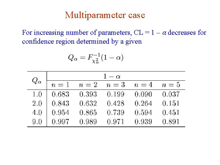
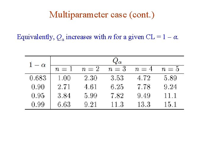
Multiparameter case For increasing number of parameters, CL = 1 – α decreases for confidence region determined by a given G. Cowan DESY Terascale School of Statistics / 19 -23 Feb 2018 / Day 2 47

Multiparameter case (cont. ) Equivalently, Qα increases with n for a given CL = 1 – α. G. Cowan DESY Terascale School of Statistics / 19 -23 Feb 2018 / Day 2 48

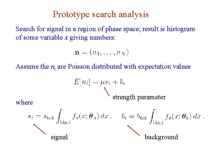
Prototype search analysis Search for signal in a region of phase space; result is histogram of some variable x giving numbers: Assume the ni are Poisson distributed with expectation values strength parameter where signal G. Cowan background DESY Terascale School of Statistics / 19 -23 Feb 2018 / Day 2 49

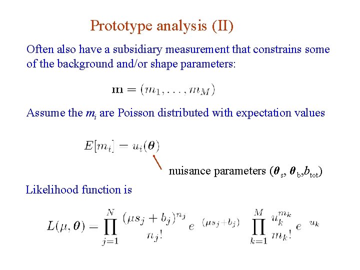
Prototype analysis (II) Often also have a subsidiary measurement that constrains some of the background and/or shape parameters: Assume the mi are Poisson distributed with expectation values nuisance parameters (θ s, θ b, btot) Likelihood function is G. Cowan DESY Terascale School of Statistics / 19 -23 Feb 2018 / Day 2 50

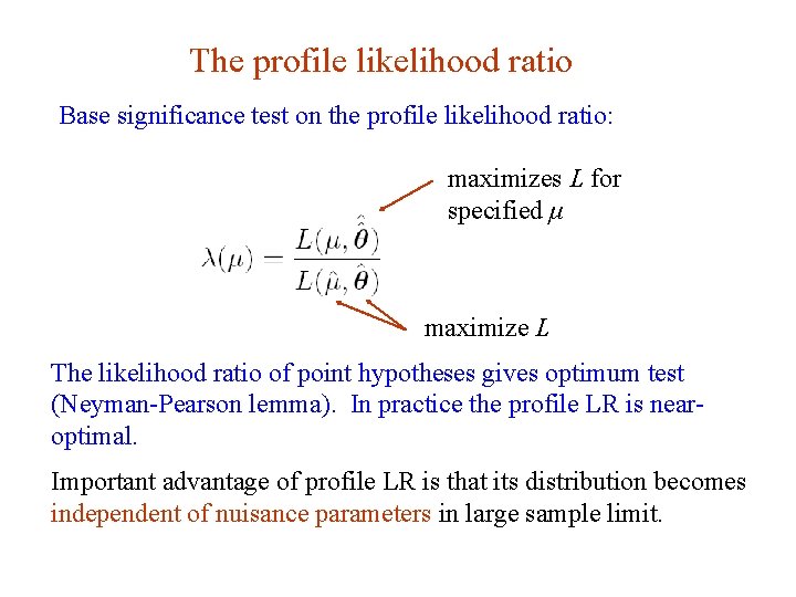
The profile likelihood ratio Base significance test on the profile likelihood ratio: maximizes L for specified μ maximize L The likelihood ratio of point hypotheses gives optimum test (Neyman-Pearson lemma). In practice the profile LR is nearoptimal. Important advantage of profile LR is that its distribution becomes independent of nuisance parameters in large sample limit. G. Cowan DESY Terascale School of Statistics / 19 -23 Feb 2018 / Day 2 51

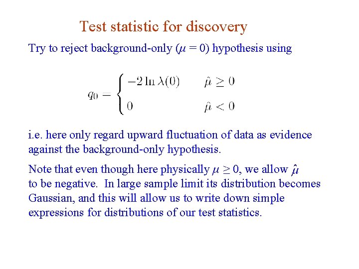
Test statistic for discovery Try to reject background-only (μ = 0) hypothesis using i. e. here only regard upward fluctuation of data as evidence against the background-only hypothesis. Note that even though here physically μ ≥ 0, we allow to be negative. In large sample limit its distribution becomes Gaussian, and this will allow us to write down simple expressions for distributions of our test statistics. G. Cowan DESY Terascale School of Statistics / 19 -23 Feb 2018 / Day 2 52

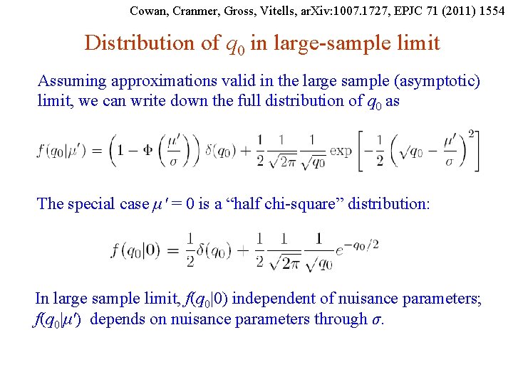
Cowan, Cranmer, Gross, Vitells, ar. Xiv: 1007. 1727, EPJC 71 (2011) 1554 Distribution of q 0 in large-sample limit Assuming approximations valid in the large sample (asymptotic) limit, we can write down the full distribution of q 0 as The special case μ′ = 0 is a “half chi-square” distribution: In large sample limit, f(q 0|0) independent of nuisance parameters; f(q 0|μ′) depends on nuisance parameters through σ. G. Cowan DESY Terascale School of Statistics / 19 -23 Feb 2018 / Day 2 53

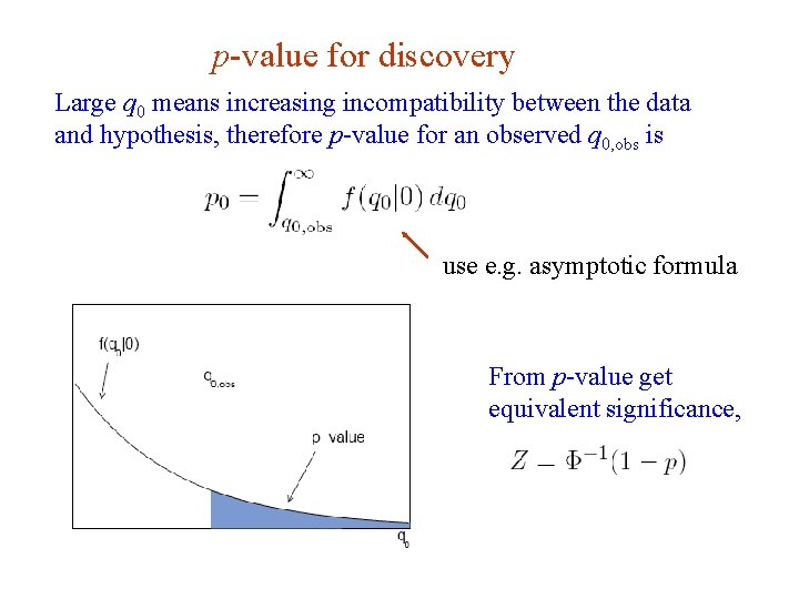
p-value for discovery Large q 0 means increasing incompatibility between the data and hypothesis, therefore p-value for an observed q 0, obs is use e. g. asymptotic formula From p-value get equivalent significance, G. Cowan DESY Terascale School of Statistics / 19 -23 Feb 2018 / Day 2 54

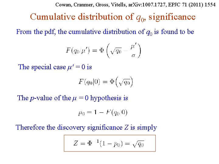
Cowan, Cranmer, Gross, Vitells, ar. Xiv: 1007. 1727, EPJC 71 (2011) 1554 Cumulative distribution of q 0, significance From the pdf, the cumulative distribution of q 0 is found to be The special case μ′ = 0 is The p-value of the μ = 0 hypothesis is Therefore the discovery significance Z is simply G. Cowan DESY Terascale School of Statistics / 19 -23 Feb 2018 / Day 2 55

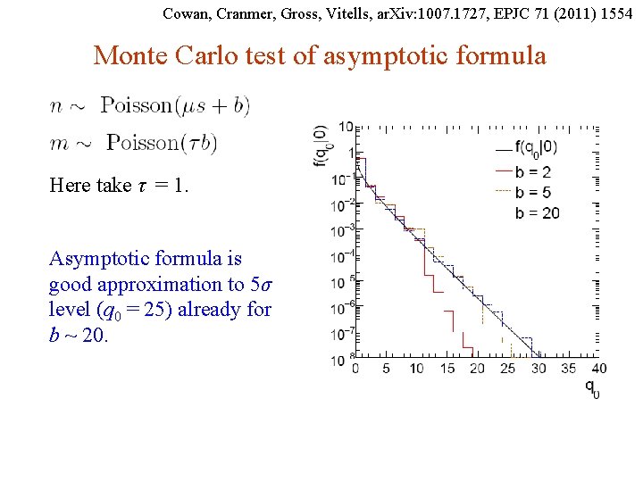
Cowan, Cranmer, Gross, Vitells, ar. Xiv: 1007. 1727, EPJC 71 (2011) 1554 Monte Carlo test of asymptotic formula Here take τ = 1. Asymptotic formula is good approximation to 5σ level (q 0 = 25) already for b ~ 20. G. Cowan DESY Terascale School of Statistics / 19 -23 Feb 2018 / Day 2 56

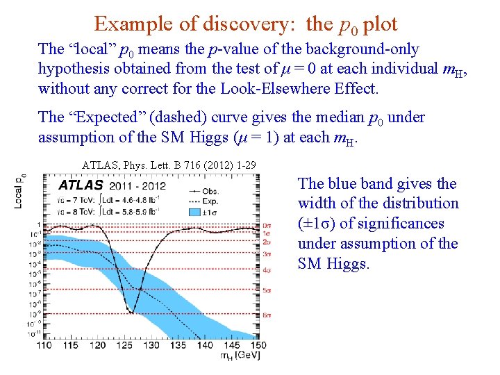
Example of discovery: the p 0 plot The “local” p 0 means the p-value of the background-only hypothesis obtained from the test of μ = 0 at each individual m. H, without any correct for the Look-Elsewhere Effect. The “Expected” (dashed) curve gives the median p 0 under assumption of the SM Higgs (μ = 1) at each m. H. ATLAS, Phys. Lett. B 716 (2012) 1 -29 The blue band gives the width of the distribution (± 1σ) of significances under assumption of the SM Higgs. G. Cowan DESY Terascale School of Statistics / 19 -23 Feb 2018 / Day 2 57

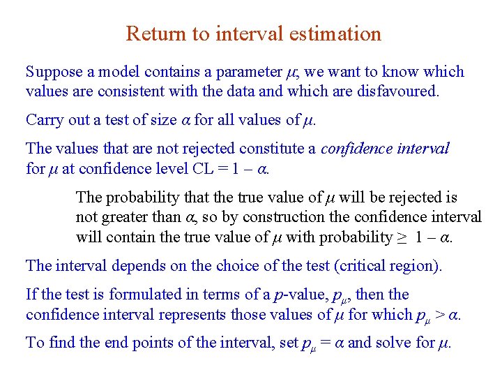
Return to interval estimation Suppose a model contains a parameter μ; we want to know which values are consistent with the data and which are disfavoured. Carry out a test of size α for all values of μ. The values that are not rejected constitute a confidence interval for μ at confidence level CL = 1 – α. The probability that the true value of μ will be rejected is not greater than α, so by construction the confidence interval will contain the true value of μ with probability ≥ 1 – α. The interval depends on the choice of the test (critical region). If the test is formulated in terms of a p-value, pμ, then the confidence interval represents those values of μ for which pμ > α. To find the end points of the interval, set pμ = α and solve for μ. G. Cowan DESY Terascale School of Statistics / 19 -23 Feb 2018 / Day 2 58

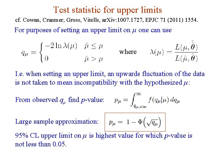
Test statistic for upper limits cf. Cowan, Cranmer, Gross, Vitells, ar. Xiv: 1007. 1727, EPJC 71 (2011) 1554. For purposes of setting an upper limit on μ one can use where I. e. when setting an upper limit, an upwards fluctuation of the data is not taken to mean incompatibility with the hypothesized μ: From observed qμ find p-value: Large sample approximation: 95% CL upper limit on μ is highest value for which p-value is not less than 0. 05. G. Cowan DESY Terascale School of Statistics / 19 -23 Feb 2018 / Day 2 59

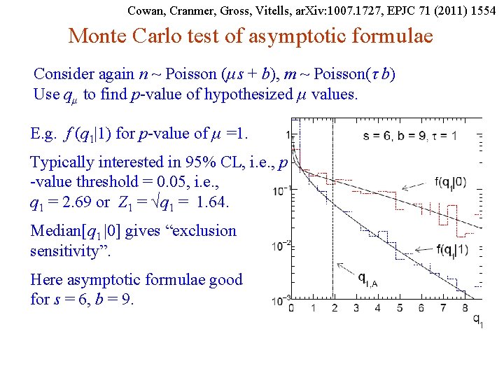
Cowan, Cranmer, Gross, Vitells, ar. Xiv: 1007. 1727, EPJC 71 (2011) 1554 Monte Carlo test of asymptotic formulae Consider again n ~ Poisson (μs + b), m ~ Poisson(τ b) Use qμ to find p-value of hypothesized μ values. E. g. f (q 1|1) for p-value of μ =1. Typically interested in 95% CL, i. e. , p -value threshold = 0. 05, i. e. , q 1 = 2. 69 or Z 1 = √q 1 = 1. 64. Median[q 1 |0] gives “exclusion sensitivity”. Here asymptotic formulae good for s = 6, b = 9. G. Cowan DESY Terascale School of Statistics / 19 -23 Feb 2018 / Day 2 60

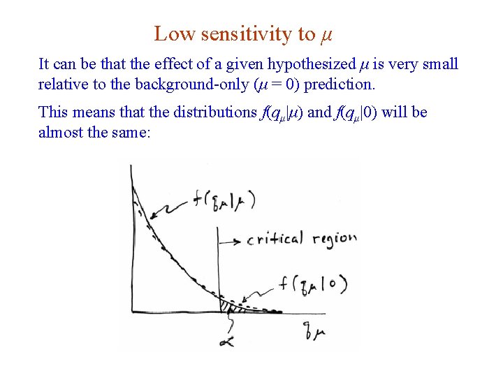
Low sensitivity to μ It can be that the effect of a given hypothesized μ is very small relative to the background-only (μ = 0) prediction. This means that the distributions f(qμ|μ) and f(qμ|0) will be almost the same: G. Cowan DESY Terascale School of Statistics / 19 -23 Feb 2018 / Day 2 61

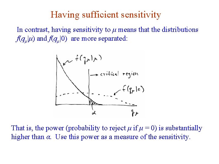
Having sufficient sensitivity In contrast, having sensitivity to μ means that the distributions f(qμ|μ) and f(qμ|0) are more separated: That is, the power (probability to reject μ if μ = 0) is substantially higher than α. Use this power as a measure of the sensitivity. G. Cowan DESY Terascale School of Statistics / 19 -23 Feb 2018 / Day 2 62

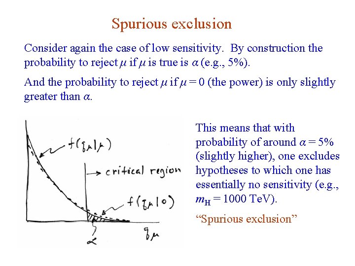
Spurious exclusion Consider again the case of low sensitivity. By construction the probability to reject μ if μ is true is α (e. g. , 5%). And the probability to reject μ if μ = 0 (the power) is only slightly greater than α. This means that with probability of around α = 5% (slightly higher), one excludes hypotheses to which one has essentially no sensitivity (e. g. , m. H = 1000 Te. V). “Spurious exclusion” G. Cowan DESY Terascale School of Statistics / 19 -23 Feb 2018 / Day 2 63

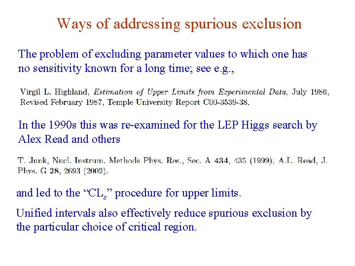
Ways of addressing spurious exclusion The problem of excluding parameter values to which one has no sensitivity known for a long time; see e. g. , In the 1990 s this was re-examined for the LEP Higgs search by Alex Read and others and led to the “CLs” procedure for upper limits. Unified intervals also effectively reduce spurious exclusion by the particular choice of critical region. G. Cowan DESY Terascale School of Statistics / 19 -23 Feb 2018 / Day 2 64

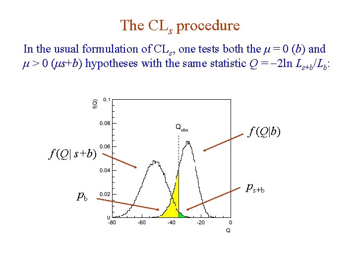
The CLs procedure In the usual formulation of CLs, one tests both the μ = 0 (b) and μ > 0 (μs+b) hypotheses with the same statistic Q = -2 ln Ls+b/Lb: f (Q|b) f (Q| s+b) pb G. Cowan ps+b DESY Terascale School of Statistics / 19 -23 Feb 2018 / Day 2 65

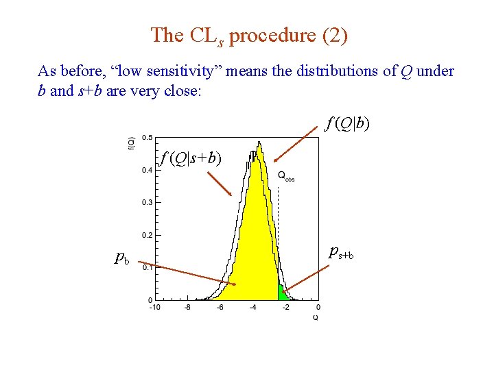
The CLs procedure (2) As before, “low sensitivity” means the distributions of Q under b and s+b are very close: f (Q|b) f (Q|s+b) pb G. Cowan ps+b DESY Terascale School of Statistics / 19 -23 Feb 2018 / Day 2 66

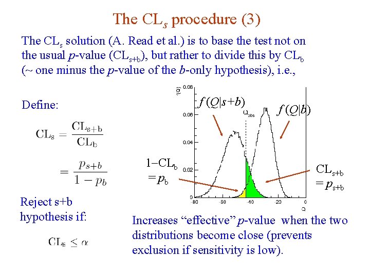
The CLs procedure (3) The CLs solution (A. Read et al. ) is to base the test not on the usual p-value (CLs+b), but rather to divide this by CLb (~ one minus the p-value of the b-only hypothesis), i. e. , f (Q|s+b) Define: 1 -CLb = pb Reject s+b hypothesis if: G. Cowan f (Q|b) CLs+b = ps+b Increases “effective” p-value when the two distributions become close (prevents exclusion if sensitivity is low). DESY Terascale School of Statistics / 19 -23 Feb 2018 / Day 2 67

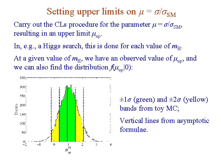
Setting upper limits on μ = σ/σSM Carry out the CLs procedure for the parameter μ = σ/σSM, resulting in an upper limit μup. In, e. g. , a Higgs search, this is done for each value of m. H. At a given value of m. H, we have an observed value of μup, and we can also find the distribution f(μup|0): ± 1σ (green) and ± 2σ (yellow) bands from toy MC; Vertical lines from asymptotic formulae. G. Cowan DESY Terascale School of Statistics / 19 -23 Feb 2018 / Day 2 68

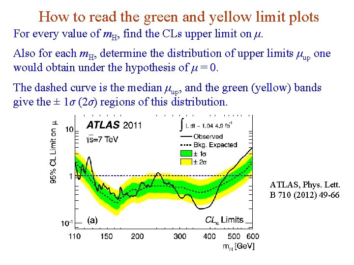
How to read the green and yellow limit plots For every value of m. H, find the CLs upper limit on μ. Also for each m. H, determine the distribution of upper limits μup one would obtain under the hypothesis of μ = 0. The dashed curve is the median μup, and the green (yellow) bands give the ± 1σ (2σ) regions of this distribution. ATLAS, Phys. Lett. B 710 (2012) 49 -66 G. Cowan DESY Terascale School of Statistics / 19 -23 Feb 2018 / Day 2 69

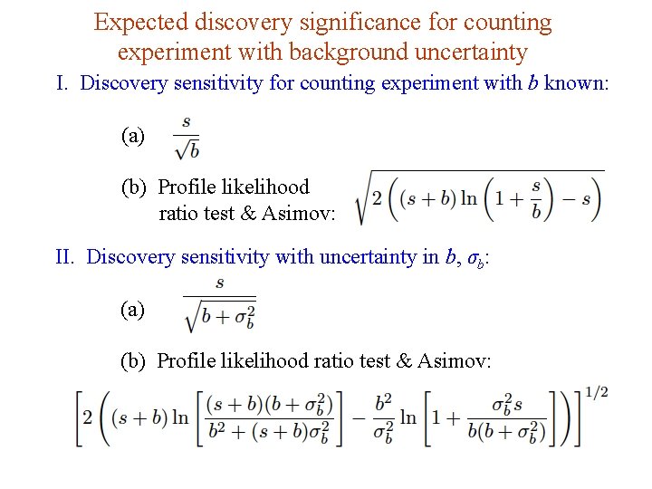
Expected discovery significance for counting experiment with background uncertainty I. Discovery sensitivity for counting experiment with b known: (a) (b) Profile likelihood ratio test & Asimov: II. Discovery sensitivity with uncertainty in b, σb: (a) (b) Profile likelihood ratio test & Asimov: G. Cowan DESY Terascale School of Statistics / 19 -23 Feb 2018 / Day 2 70

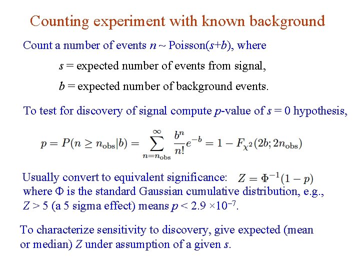
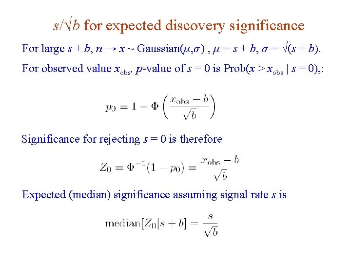
Counting experiment with known background Count a number of events n ~ Poisson(s+b), where s = expected number of events from signal, b = expected number of background events. To test for discovery of signal compute p-value of s = 0 hypothesis, Usually convert to equivalent significance: where Φ is the standard Gaussian cumulative distribution, e. g. , Z > 5 (a 5 sigma effect) means p < 2. 9 × 10 -7. To characterize sensitivity to discovery, give expected (mean or median) Z under assumption of a given s. G. Cowan DESY Terascale School of Statistics / 19 -23 Feb 2018 / Day 2 71

s/√b for expected discovery significance For large s + b, n → x ~ Gaussian(μ, σ ) , μ = s + b, σ = √(s + b). For observed value xobs, p-value of s = 0 is Prob(x > xobs | s = 0), : Significance for rejecting s = 0 is therefore Expected (median) significance assuming signal rate s is G. Cowan DESY Terascale School of Statistics / 19 -23 Feb 2018 / Day 2 72

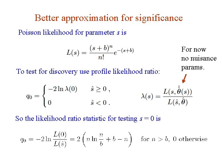
Better approximation for significance Poisson likelihood for parameter s is To test for discovery use profile likelihood ratio: For now no nuisance params. So the likelihood ratio statistic for testing s = 0 is G. Cowan DESY Terascale School of Statistics / 19 -23 Feb 2018 / Day 2 73

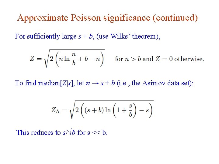
Approximate Poisson significance (continued) For sufficiently large s + b, (use Wilks’ theorem), To find median[Z|s], let n → s + b (i. e. , the Asimov data set): This reduces to s/√b for s << b. G. Cowan DESY Terascale School of Statistics / 19 -23 Feb 2018 / Day 2 74

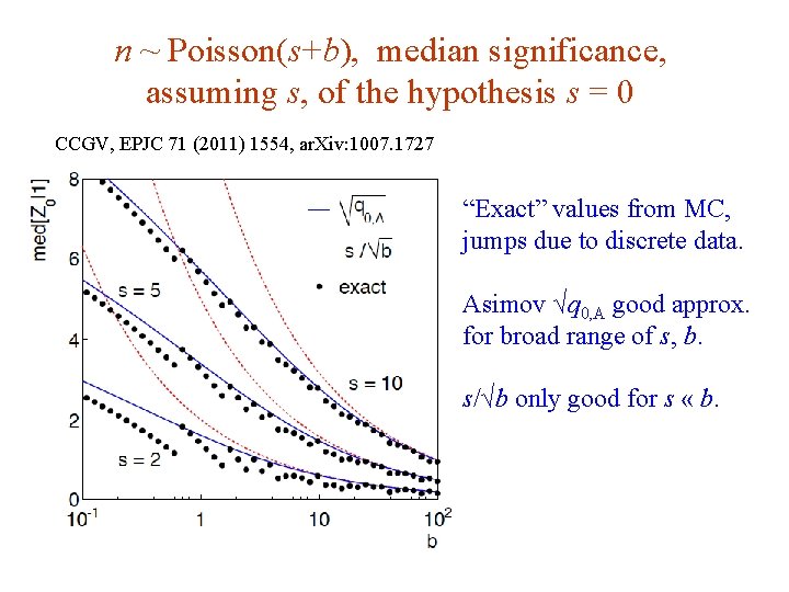
n ~ Poisson(s+b), median significance, assuming s, of the hypothesis s = 0 CCGV, EPJC 71 (2011) 1554, ar. Xiv: 1007. 1727 “Exact” values from MC, jumps due to discrete data. Asimov √q 0, A good approx. for broad range of s, b. s/√b only good for s « b. G. Cowan DESY Terascale School of Statistics / 19 -23 Feb 2018 / Day 2 75

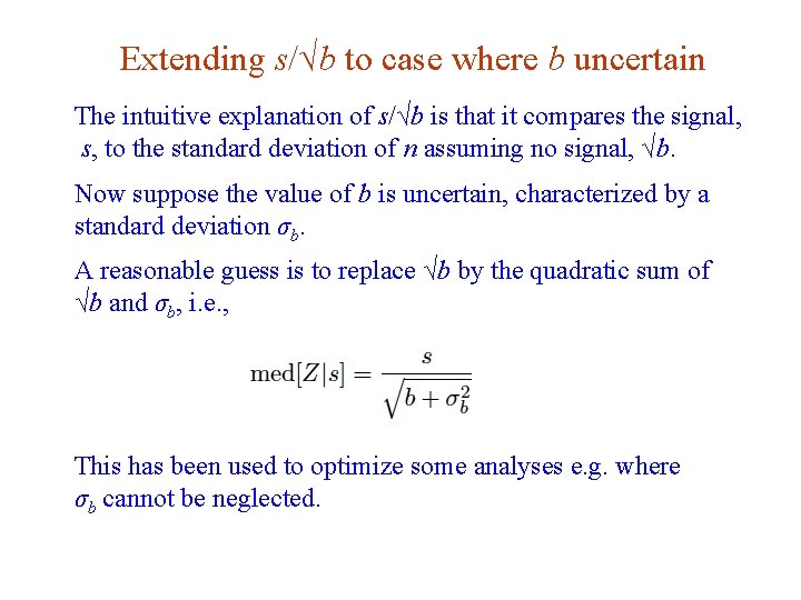
Extending s/√b to case where b uncertain The intuitive explanation of s/√b is that it compares the signal, s, to the standard deviation of n assuming no signal, √b. Now suppose the value of b is uncertain, characterized by a standard deviation σb. A reasonable guess is to replace √b by the quadratic sum of √b and σb, i. e. , This has been used to optimize some analyses e. g. where σb cannot be neglected. G. Cowan DESY Terascale School of Statistics / 19 -23 Feb 2018 / Day 2 76

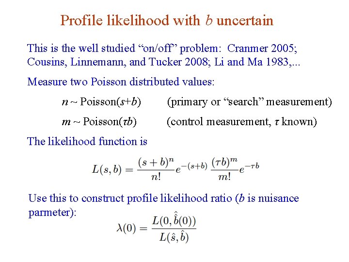
Profile likelihood with b uncertain This is the well studied “on/off” problem: Cranmer 2005; Cousins, Linnemann, and Tucker 2008; Li and Ma 1983, . . . Measure two Poisson distributed values: n ~ Poisson(s+b) (primary or “search” measurement) m ~ Poisson(τb) (control measurement, τ known) The likelihood function is Use this to construct profile likelihood ratio (b is nuisance parmeter): G. Cowan DESY Terascale School of Statistics / 19 -23 Feb 2018 / Day 2 77

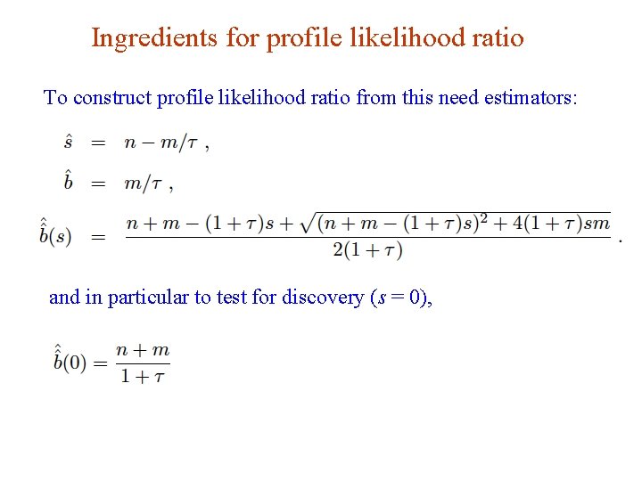
Ingredients for profile likelihood ratio To construct profile likelihood ratio from this need estimators: and in particular to test for discovery (s = 0), G. Cowan DESY Terascale School of Statistics / 19 -23 Feb 2018 / Day 2 78

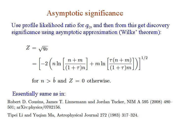
Asymptotic significance Use profile likelihood ratio for q 0, and then from this get discovery significance using asymptotic approximation (Wilks’ theorem): Essentially same as in: G. Cowan DESY Terascale School of Statistics / 19 -23 Feb 2018 / Day 2 79

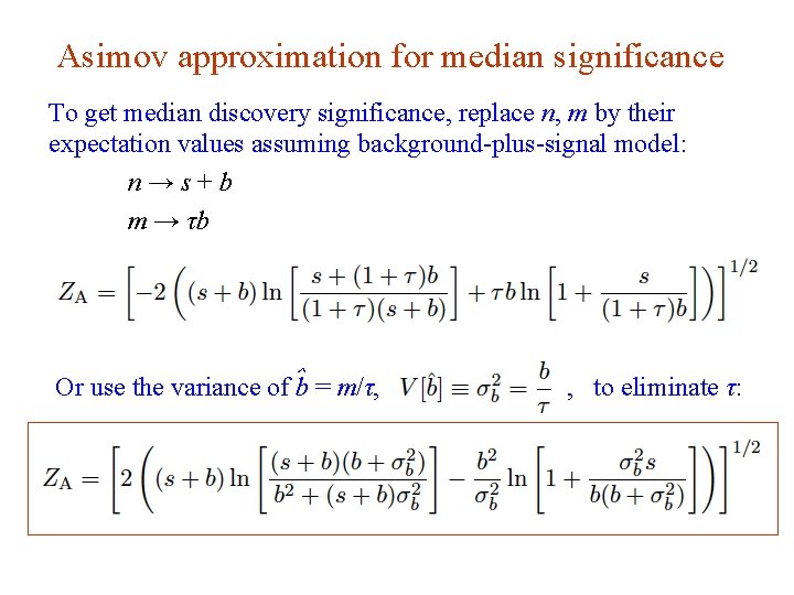
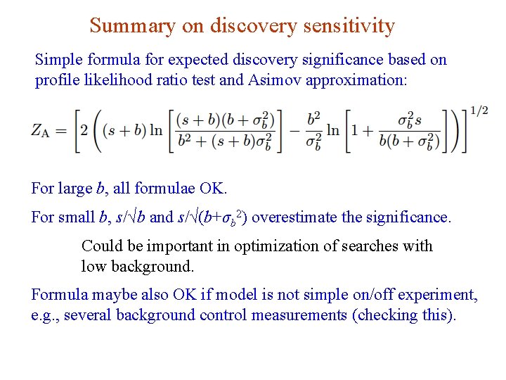
Asimov approximation for median significance To get median discovery significance, replace n, m by their expectation values assuming background-plus-signal model: n→s+b m → τb Or use the variance of ˆb = m/τ, G. Cowan , to eliminate τ: DESY Terascale School of Statistics / 19 -23 Feb 2018 / Day 2 80

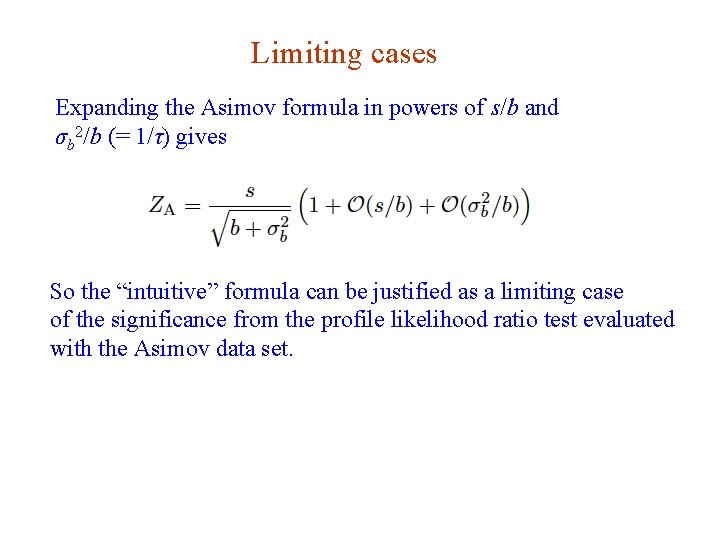
Limiting cases Expanding the Asimov formula in powers of s/b and σb 2/b (= 1/τ) gives So the “intuitive” formula can be justified as a limiting case of the significance from the profile likelihood ratio test evaluated with the Asimov data set. G. Cowan DESY Terascale School of Statistics / 19 -23 Feb 2018 / Day 2 81

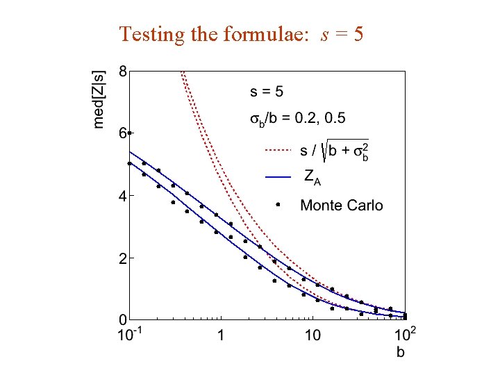
Testing the formulae: s = 5 G. Cowan DESY Terascale School of Statistics / 19 -23 Feb 2018 / Day 2 82

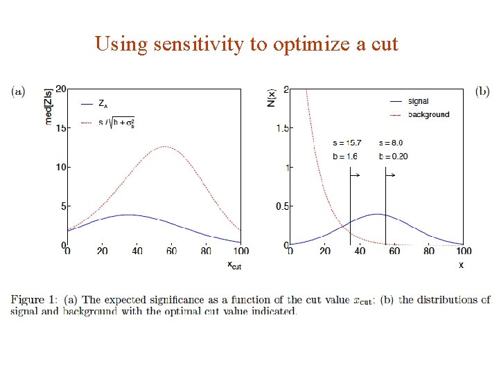
Using sensitivity to optimize a cut G. Cowan DESY Terascale School of Statistics / 19 -23 Feb 2018 / Day 2 83

Summary on discovery sensitivity Simple formula for expected discovery significance based on profile likelihood ratio test and Asimov approximation: For large b, all formulae OK. For small b, s/√b and s/√(b+σb 2) overestimate the significance. Could be important in optimization of searches with low background. Formula maybe also OK if model is not simple on/off experiment, e. g. , several background control measurements (checking this). G. Cowan DESY Terascale School of Statistics / 19 -23 Feb 2018 / Day 2 84

Finally Four lectures only enough for a brief introduction to: Parameter estimation Unfolding Statistical tests for discovery and limits Experimental sensitivity Many other important topics; some covered in rest of week: Bayesian methods, MCMC Multivariate methods, Machine Learning The look-elsewhere effect, etc. Final thought: once the basic formalism is understood, most of the work focuses on building the model, i. e. , writing down the likelihood, e. g. , P(x|θ), and including in it enough parameters to adequately describe the data (true for both Bayesian and frequentist approaches). G. Cowan DESY Terascale School of Statistics / 19 -23 Feb 2018 / Day 2 85

Extra slides G. Cowan DESY Terascale School of Statistics / 19 -23 Feb 2018 / Day 2 86

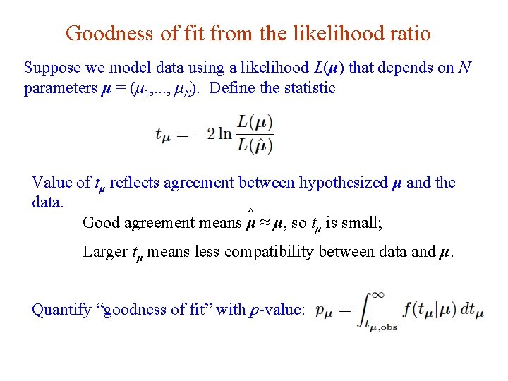
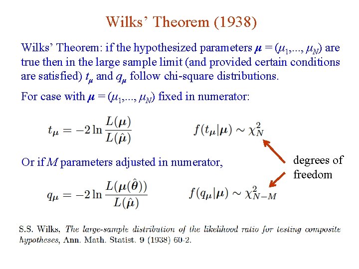
Goodness of fit from the likelihood ratio Suppose we model data using a likelihood L(μ) that depends on N parameters μ = (μ 1, . . . , μΝ). Define the statistic Value of tμ reflects agreement between hypothesized μ and the data. ⌃ Good agreement means μ ≈ μ, so tμ is small; Larger tμ means less compatibility between data and μ. Quantify “goodness of fit” with p-value: G. Cowan DESY Terascale School of Statistics / 19 -23 Feb 2018 / Day 2 87

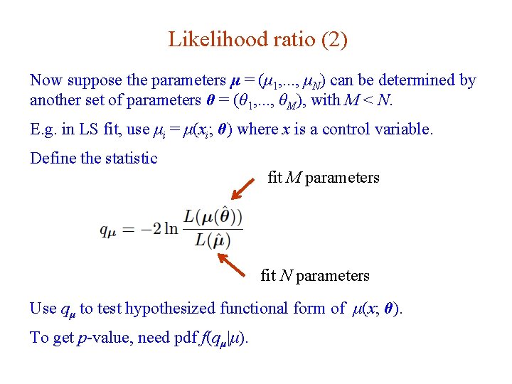
Likelihood ratio (2) Now suppose the parameters μ = (μ 1, . . . , μΝ) can be determined by another set of parameters θ = (θ 1, . . . , θM), with M < N. E. g. in LS fit, use μi = μ(xi; θ) where x is a control variable. Define the statistic fit M parameters fit N parameters Use qμ to test hypothesized functional form of μ(x; θ). To get p-value, need pdf f(qμ|μ). G. Cowan DESY Terascale School of Statistics / 19 -23 Feb 2018 / Day 2 88

Wilks’ Theorem (1938) Wilks’ Theorem: if the hypothesized parameters μ = (μ 1, . . . , μΝ) are true then in the large sample limit (and provided certain conditions are satisfied) tμ and qμ follow chi-square distributions. For case with μ = (μ 1, . . . , μΝ) fixed in numerator: Or if M parameters adjusted in numerator, G. Cowan DESY Terascale School of Statistics / 19 -23 Feb 2018 / Day 2 degrees of freedom 89

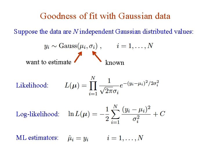
Goodness of fit with Gaussian data Suppose the data are N independent Gaussian distributed values: want to estimate known Likelihood: Log-likelihood: ML estimators: G. Cowan DESY Terascale School of Statistics / 19 -23 Feb 2018 / Day 2 90

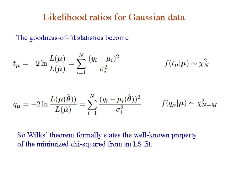
Likelihood ratios for Gaussian data The goodness-of-fit statistics become So Wilks’ theorem formally states the well-known property of the minimized chi-squared from an LS fit. G. Cowan DESY Terascale School of Statistics / 19 -23 Feb 2018 / Day 2 91

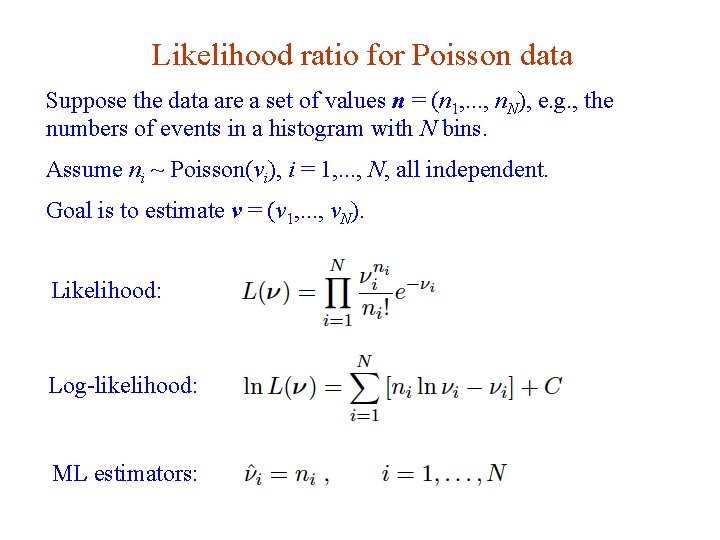
Likelihood ratio for Poisson data Suppose the data are a set of values n = (n 1, . . . , nΝ), e. g. , the numbers of events in a histogram with N bins. Assume ni ~ Poisson(νi), i = 1, . . . , N, all independent. Goal is to estimate ν = (ν 1, . . . , νΝ). Likelihood: Log-likelihood: ML estimators: G. Cowan DESY Terascale School of Statistics / 19 -23 Feb 2018 / Day 2 92

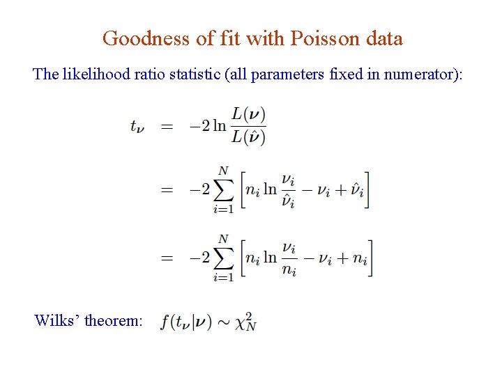
Goodness of fit with Poisson data The likelihood ratio statistic (all parameters fixed in numerator): Wilks’ theorem: G. Cowan DESY Terascale School of Statistics / 19 -23 Feb 2018 / Day 2 93

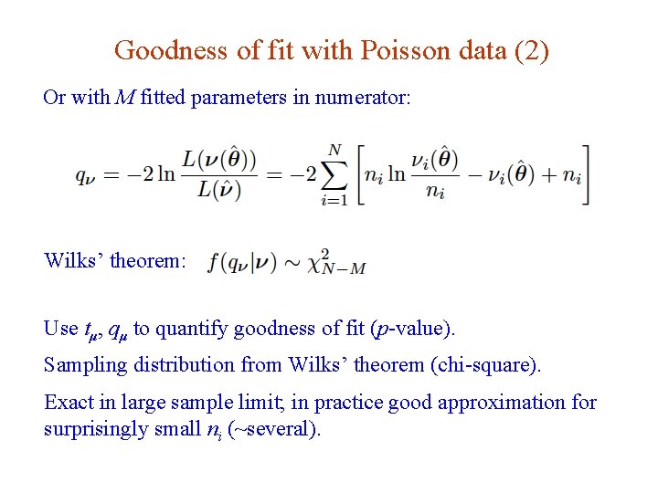
Goodness of fit with Poisson data (2) Or with M fitted parameters in numerator: Wilks’ theorem: Use tμ, qμ to quantify goodness of fit (p-value). Sampling distribution from Wilks’ theorem (chi-square). Exact in large sample limit; in practice good approximation for surprisingly small ni (~several). G. Cowan DESY Terascale School of Statistics / 19 -23 Feb 2018 / Day 2 94

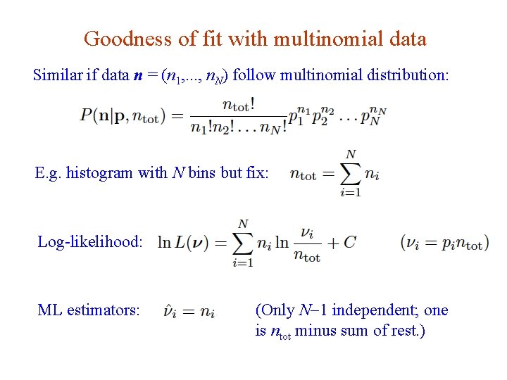
Goodness of fit with multinomial data Similar if data n = (n 1, . . . , nΝ) follow multinomial distribution: E. g. histogram with N bins but fix: Log-likelihood: ML estimators: G. Cowan (Only N-1 independent; one is ntot minus sum of rest. ) DESY Terascale School of Statistics / 19 -23 Feb 2018 / Day 2 95

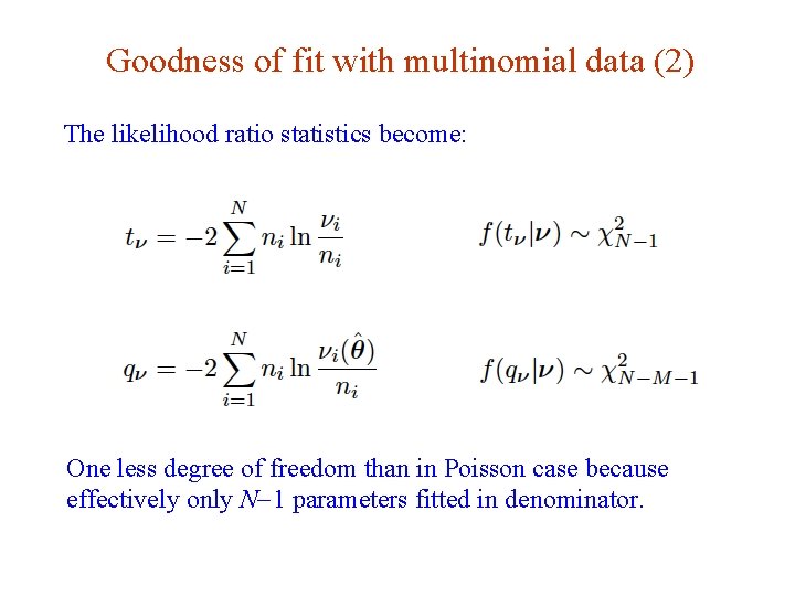
Goodness of fit with multinomial data (2) The likelihood ratio statistics become: One less degree of freedom than in Poisson case because effectively only N-1 parameters fitted in denominator. G. Cowan DESY Terascale School of Statistics / 19 -23 Feb 2018 / Day 2 96

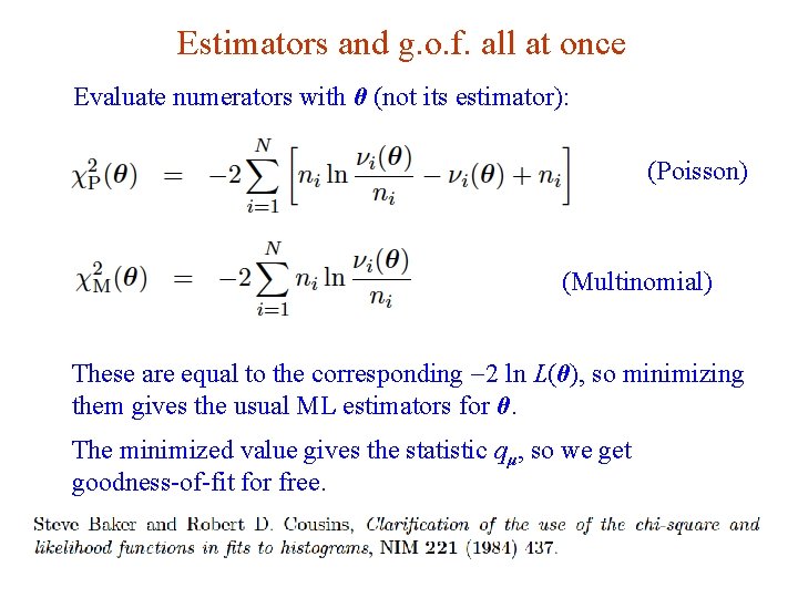
Estimators and g. o. f. all at once Evaluate numerators with θ (not its estimator): (Poisson) (Multinomial) These are equal to the corresponding -2 ln L(θ), so minimizing them gives the usual ML estimators for θ. The minimized value gives the statistic qμ, so we get goodness-of-fit for free. G. Cowan DESY Terascale School of Statistics / 19 -23 Feb 2018 / Day 2 97