ECON 214 Statistics for Economists Course OutlineSecond Semester

• • ECON 214: Statistics for Economists Course Outline—Second Semester 2015/2016 Instructors: 1. Dr. K. A. Tutu 2. Mr Theodore O. Antwi-Asare 3. Dr B. Senadza Email: toasare@ug. edu. gh Office hours: Tuesdays 10: 30 am- 1: 00 pm-Or By appointment Copyright © 2004 Pearson Education, Inc.

Definition v. Statistics is the science that deals with methods and procedures to collect, organize, summarize, analyze, and draw conclusions from data. v Copyright © 2004 Pearson Education, Inc.

• STATISTICS is concerned with scientific methods for collecting, organising, summarising, presenting and analysing data, as well as, drawing valid conclusions and making reasonable decisions on the basis of such analysis.

• In a narrower sense, the term statistics is used to denote the data themselves or the numbers derived from the data such as averages, thus • we speak about Balance of payments Statistics; employment statistics; accident statistics; economic statistics etc.

STATISTICS v Descriptive Statistics summarize or describe the important characteristics of a known set of data v Inferential Statistics use sample data to make inferences (or generalizations) about a population

Definitions v Data observations numerical or otherwise (such as measurements, survey responses) that have been collected. Copyright © 2004 Pearson Education, Inc.

Definitions v. Population the complete collection of all elements (scores, people, measurements, and so on) to be studied. The collection is complete in the sense that it includes all subjects to be studied. Copyright © 2004 Pearson Education, Inc.

v. Census Definitions the collection of data from every member of the population. v. Sample a sub-collection of elements drawn from a population. Copyright © 2004 Pearson Education, Inc.

Key Concepts Sample data must be collected in an appropriate way, such as through a process of random selection. v v If sample data are not collected in an appropriate way, the data may be so completely useless that no amount of statistical torturing can salvage them.

Definitions v. Quantitative data numbers representing counts or measurements. Example: weights of students. Copyright © 2004 Pearson Education, Inc.

Definitions v Qualitative (or categorical or attribute) data can be separated into different categories that are distinguished by some nonnumeric characteristics. Example: gender (male/female) of athletes; colour; ethnic group etc

Working with Quantitative Data Quantitative data can further be distinguished between discrete and continuous types. Copyright © 2004 Pearson Education, Inc.

Definitions v. Discrete data result when the number of possible values is either a finite number or a ‘countable’ number of possible values. 0, 1, 2, 3, . . . Example: The number of eggs that hens lay. Copyright © 2004 Pearson Education, Inc.

Definitions v. Continuous (numerical) data result from infinitely many possible values that correspond to some continuous scale that covers a range of values without gaps, interruptions, or jumps. 2 3 Example: The amount of milk that a cow produces; e. g. 2. 343115 gallons Copyright © 2004 Pearson Education, Inc.

Levels of Measurement Another way to classify data is to use levels of measurement. FOUR of these levels are discussed in the following slides.

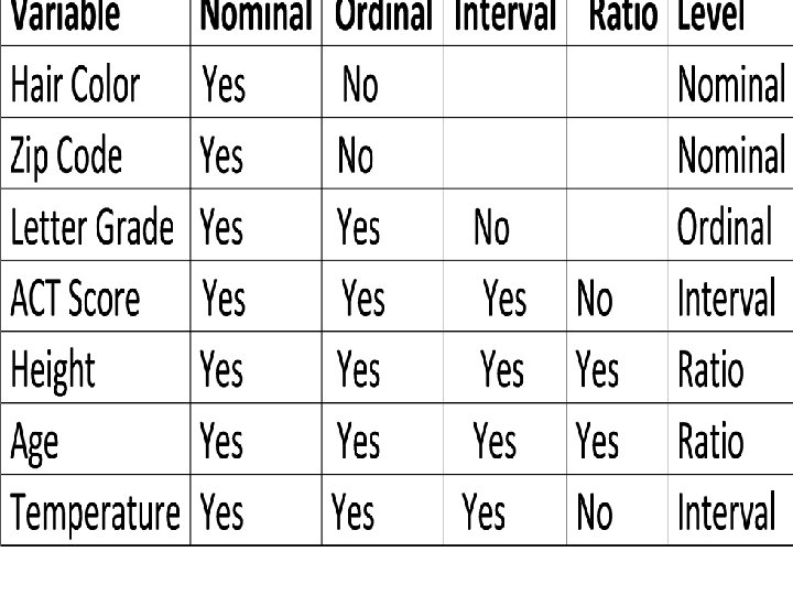
Definitions v Nominal level of measurement characterized by data that consist of names, labels, or categories only. The data cannot be arranged in an ordering scheme (such as low to high) Example: survey responses yes, no, undecided Copyright © 2004 Pearson Education, Inc.

Definitions v Ordinal level of measurement involves data that may be arranged in some order, but differences between data values either cannot be determined or are meaningless Example: Course grades A, B, C, D, or F Copyright © 2004 Pearson Education, Inc.

Definitions v Interval level of measurement like the ordinal level, with the additional property that the difference between any two data values is meaningful. However, there is no natural zero starting point (where none of the quantity is present) Example: Years 1000, 2000, 1776, and 1492 Copyright © 2004 Pearson Education, Inc.

Definitions v Ratio level of measurement the interval level modified to include the natural zero starting point (where zero indicates that none of the quantity is present). For values at this level, differences and ratios are meaningful. Example: Prices of college textbooks ($0 represents no cost) Copyright © 2004 Pearson Education, Inc.

Summary Levels of Measurement v Nominal - categories only v Ordinal - categories with some order v Interval - differences but no natural starting point or zero v Ratio - differences and a natural starting point (zero) Copyright © 2004 Pearson Education, Inc.

Levels of Measurement 1. Nominal – categorical (names) 2. Ordinal – nominal, plus can be ranked (order) 3. Interval – ordinal, plus intervals are consistent (differences but no natural zero starting point) 4. Ratio – interval, plus ratios are consistent, true zero (difference and a natural zero starting point)

Recap We have looked at: Basic definitions and terms describing data v Parameters versus statistics v Types of data (quantitative and qualitative) v Levels of measurement Copyright © 2004 Pearson Education, Inc.

Section 1 -3 Critical Thinking

• METHODS OF RANDM SAMPLING • Random sampling is a type of sampling in which every item in a population of interest, or target population, has a known, and usually equal, chance of being chosen for inclusion in the sample. • Having such a sample ensures that the sample items are chosen without bias and provides the statistical basis for determining the confidence that can be associated with the inferences. A random sample is also called a probability sample, or scientific sample.

• The four principal methods of random sampling are the simple, systematic, stratified, and cluster sampling methods. A simple random sample is one in which individual items are chosen from the target population on the basis of chance. • Such chance selection is similar to the random drawing of numbers in a lottery. However, in statistical sampling a table of random numbers or a random-number generator computer program generally is used to identify the numbered items in the population that are to be selected for the sample.

Success in Statistics v Success in the introductory statistics course typically requires more common sense than mathematical expertise. v This section is designed to illustrate how common sense is used when we think critically about data and statistics. Copyright © 2004 Pearson Education, Inc.

Misuses of Statistics v. Bad Samples v. Small Samples v. Misleading Graphs v. Pictographs v. Distorted Percentages v. Loaded Questions v. Order of Questions Copyright © 2004 Pearson Education, v. Refusals v. Correlation & Causality v. Self Interest Study v. Precise Numbers v. Partial Pictures v. Deliberate Distortions

Definitions v Voluntary response sample (or self-selected survey) one in which the respondents themselves decide whether to be included. In this case, valid conclusions can be made only about the specific group of people who agree to participate. Copyright © 2004 Pearson Education, Inc.

Misleading Graphs Copyright © 2004 Pearson Education, Inc.

To correctly interpret a graph, we should analyze the numerical information given in the graph instead of being mislead by its general shape. Copyright © 2004 Pearson Education, Inc.

Misuses of Statistics v Bad Samples v Small Samples v Misleading Graphs v Pictographs/Pictograms Copyright © 2004 Pearson Education, Inc.

Double the length, width, and height of a cube, and the volume increases by a factor of eight Figure 1 -2 Copyright © 2004 Pearson Education, Inc.

Misuses of Statistics v. Bad Samples v. Small Samples v. Misleading Graphs v. Pictographs v. Distorted Percentages v. Loaded Questions v. Order of Questions Copyright © 2004 Pearson Education, Inc. v. Refusals v. Correlation & Causality v. Self Interest Study v. Precise Numbers v. Partial Pictures v. Deliberate Distortions

Recap In this section we have: v Reviewed 13 misuses of statistics. v Illustrated how common sense can play a big role in interpreting data and statistics Copyright © 2004 Pearson Education, Inc.

Major Points v If sample data are not collected in an appropriate way, the data may be so completely useless that no amount of statistical tutoring can salvage them. v Randomness typically plays a critical role in determining which data to collect. Copyright © 2004 Pearson Education, Inc.

Definitions v Observational Study observing and measuring specific characteristics without attempting to modify the subjects being studied Copyright © 2004 Pearson Education, Inc.

Definitions v Experiment apply some treatment and then observe its effects on the subjects Copyright © 2004 Pearson Education, Inc.

Definitions v Cross Sectional Study Data are observed, measured, and collected at one point in time. v Retrospective (or Case Control) Study Data are collected from the past by going back in time. v Prospective (or Longitudinal or Cohort) Study Data are collected into the future from groups (called cohorts) sharing common factors. Copyright © 2004 Pearson Education, Inc.

Definitions v Confounding occurs in an experiment when the experimenter is not able to distinguish between the effects of different factors Try to plan the experiment so confounding does not occur! Copyright © 2004 Pearson Education, Inc.

Controlling Effects of Variables v Blinding subject does not know he or she is receiving a treatment or placebo v Blocks groups of subjects with similar characteristics v Completely Randomized Experimental Design subjects are put into blocks through a process of random selection v Rigorously Controlled Design subjects are very carefully chosen Copyright © 2004 Pearson Education, Inc.

Replication and Sample Size v Replication repetition of an experiment when there are enough subjects to recognize the differences in different treatments v Sample Size use a sample size that is large enough to see the true nature of any effects and obtain that sample using an appropriate method, such as one based on randomness Copyright © 2004 Pearson Education, Inc.

Definitions v Random Sample members of the population are selected in such a way that each individual member has an equal chance of being selected v. Simple Random Sample (of size n) subjects selected in such a way that every possible sample of the same size n has the same chance of being chosen Copyright © 2004 Pearson Education, Inc.

Random Sampling selection so that each has an equal chance of being selected Copyright © 2004 Pearson Education, Inc.

Systematic Sampling Select some starting point and then select every K th element in the population Copyright © 2004 Pearson Education, Inc.

Convenience Sampling use results that are easy to get Copyright © 2004 Pearson Education, Inc.

Stratified Sampling subdivide the population into at least two different subgroups that share the same characteristics, then draw a sample from each subgroup (or stratum) Copyright © 2004 Pearson Education, Inc.

Cluster Sampling divide the population into sections (or clusters); randomly select some of those clusters; choose all members from selected clusters Copyright © 2004 Pearson Education, Inc.

Methods of Sampling v Random v Systematic v Convenience v Stratified v Cluster Copyright © 2004 Pearson Education, Inc.

Definitions v Sampling Error the difference between a sample result and the true population result; such an error results from chance sample fluctuations v Nonsampling Error sample data that are incorrectly collected, recorded, or analyzed (such as by selecting a biased sample, using a defective instrument, or copying the data incorrectly) Copyright © 2004 Pearson Education, Inc.

Recap In this section we have looked at: v Types of studies and experiments v Controlling the effects of variables v Randomization v Types of sampling v Sampling Errors

DESCRIPTIVE STATISTICS

• Descriptive statistics are useful for summarising large amounts of information -highlighting the main features but omitting the detail. • Different techniques are suited to different types of data, e. g. bar charts for cross-section data and • Line graphs or rates of growth for time series.

Graphical methods, such as the bar chart, provide a picture of the data. • These give an informal summary but they MAY BE unsuitable as a basis for further analysis • Important graphical techniques include the bar chart, LINE GRAPH, frequency distribution,

• relative and cumulative frequency distributions, histogram and pie chart. • For time-series data a time-series chart of the data is informative • Numerical techniques are more precise as summaries. • Measures: of location (such as the mean); of dispersion (the variance); • and of skewness form the basis of these methods

• Important numerical summary statistics include • the mean, median and mode; • variance, standard deviation and coefficient of variation; • coefficient of skewness.

• For bivariate data the scatter diagram (or XY graph) is a useful way of illustrating the data. • Data are often transformed in some way before analysis, e. g. by taking logs. • Transformations often make it easier to see key features of the data in graphs • and sometimes make summary statistics easier to interpret

• Scatter Plot Y • Scatter diagram • Scattergram X

FREQUENCY DISTRIBUTIONS

Classes 70 61 52 43 34 25 16 – – – – 78 69 60 51 42 33 24 Class boundaries 69. 5 60. 5 51. 5 42. 5 33. 5 24. 5 15. 5 – – – – 78. 5 69. 5 60. 5 51. 5 42. 5 33. 5 24. 5 Tally Marks ///// // /////-/////-/////-// Freq. x 5 5 0 2 7 14 17 74 65 56 47 38 29 20

A frequency distribution table lists categories of scores OR data along with their corresponding frequencies.

The frequency for a particular category or class is the number of original scores that fall into that class.

The classes or categories refer to the groupings of a frequency table

• The range is the difference between the highest value and the lowest value. Range = highest value – lowest value

The class limits are the smallest or the largest numbers (data points) that can actually belong to different classes.

• Lower class limits: are the smallest numbers that can actually belong to the different classes. • Upper class limits: are the largest numbers that can actually belong to the different classes.

The class width is the difference between two consecutive lower class limits or class boundaries.

• The class boundaries are obtained by increasing the upper class limits and decreasing the lower class limits by the same amount so that there are no gaps between consecutive classes. • The amount to be added or subtracted is ½ the difference between the upper limit of one class and the lower limit of the following class.

Essential Question : • How do we construct a frequency distribution table?

Process of Constructing a Frequency Table • STEP 1: Determine the Range = Highest Value – Lowest Value from the data set

• STEP 2. Determine the tentative number of classes (k) USE k = 1 + 3. 322 log N • OR IF YOU ARE GIVEN A SPECIFIED NUMBER OF CLASSES THEN USE IT • Always round – off. Note: The number of classes should be between 5 and 20. The actual number of classes may be affected by convenience or other subjective factors

• STEP 3. Find the class width by dividing the Range by the number of classes. (Always round – off )

• STEP 4. Write the classes or categories starting with the lowest score. Stop when the class already includes the highest score. • Add the class width to the starting point to get the second lower class limit. Add the class width to the second lower class limit to get the third, and so on. List the lower class limits in a vertical column and enter the upper class limits, which can be easily identified at this stage. • STEP 5: TALLY the data and for each class add the tallies

• STEP 6. Determine the frequency for each class by referring to the sum of the tally columns and present the results in a table.

When constructing frequency tables, the following guidelines should be followed. • The classes must be mutually exclusive. That is, each score must belong to exactly one class. • Include all classes, even if the frequency might be zero.

• All classes should have the same width, although it is sometimes impossible to avoid open – ended intervals such as “ 65 years or older”. • The number of classes should be between 5 and 20.

Let’s Try!!! • Time magazine collected information on all 464 people who died from gunfire in the Philippines during one week. Here are the ages of 50 men randomly selected from that population. Construct a frequency distribution table.

19 23 47 17 24 21 27 18 25 69 36 29 27 23 30 21 20 65 42 23 40 41 33 73 25 33 65 17 20 76 31 18 24 35 24 70 22 25 65 16 37 26 46 27 63 25 71 37 75 25

Using Table: • What is the lower class limit of the highest class? Upper class limit of the lowest class? • Find the class mark of the class 43 – 51. • What is the frequency of the class 16 – 24?

Classes 70 – 78 61 – 69 52 – 60 43 – 51 34 – 42 25 – 33 16 – 24 Class Boundaries 69. 5 – 78. 5 60. 5 – 69. 5 51. 5 – 60. 5 42. 5 – 51. 5 33. 5 – 42. 5 24. 5 – 33. 5 15. 5 – 24. 5 Tally Freq. X //// //// // 5 5 0 2 7 14 17 74 65 56 47 38 29 20 //// //

Classes Class Mark Class Tally Boundarie s Frequency 16 – 24 20 15. 5 – 24. 5 Show 17 25 -33 29 24. 5 – 33. 5 Etc 14 34 -42 38 33. 5 – 42. 5 Etc 7 43 - 51 47 42. 5 – 51. 5 Etc 2 52 – 60 56 51. 5 – 60. 5 Etc 0 61 – 69 65 60. 5 - 69. 5 Etc 5 70 – 78 74 69. 5 – 78. 5 etc 5 50

Classes Class Mark Frequenc y 16 – 24 20 17 25 - 33 34 - 42 43 - 51 52 – 60 61 – 69 70 – 78 29 38 47 56 65 74 14 7 2 0 5 5 50

Example 1 The manager of Osino Auto would like to have a better understanding of the cost of parts used in the engine tune-ups performed in the shop. She examines 50 customer invoices for tune-ups. The costs of parts, rounded off to the nearest $, are listed below.

• CONSTRUCT A FREQUENCY DISTRIBUTION FOR THE DATA

CUMULATIVE FREQUENCY DISTRIBUTION • The less than cumulative frequency distribution (F<) is constructed by adding the frequencies from the lowest to the highest interval • while the more than cumulative frequency distribution (F>) is constructed by adding the frequencies from the highest class interval to the lowest class interval.

Tabular Summary Frequency Distribution of engine tune-ups Cumulative Frequency Cost ($) Frequency Relative Frequency less than 0. 04 2 2 50 -59 more than 50 60 -69 13 0. 26 70 -79 16 0. 32 80 -89 7 0. 14 38 90 -99 7 0. 14 45 12 100 -109 5 0. 10 50 5 50 1. 00 45 tune-ups cost less than $ 100 12 tune-ups cost more than $ 89 2 + 13 15 48 31 35 5+7 18

Ogive less than ogive Frequency 50 40 30 20 more than ogive 10 60 70 80 90 100 110 median Tune-up Cost ($)

• Relative frequency =frequency/sum of frequencies • = f/Σf • Relative frequency is used as the y axis for some Ogives and Relative frequency polygons

Frequency Density (X 10) Graphical Summary: Histogram 18 16 14 12 10 8 6 4 2 50 -59 60 -69 70 -79 80 -89 90 -99 100 -110 Cost ($) Unlike a bar graph, a histogram has no natural separation between rectangles of adjacent classes.

HISTOGRAM • A histogram is similar to a bar chart except that it corrects for differences in class widths. • If all the class widths are identical then there is no difference between a bar chart and a histogram.

• The calculations required to produce the • histogram are as follows: • The Y axis shows the frequency density which is defined as follows: • frequency density = frequency/ class width

FREQUENCY POLYGON • A frequency polygon would be the result if, instead of drawing blocks for the histogram, • one drew lines connecting the centres of the top of each block.

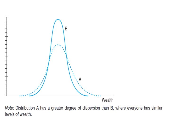
KEY STATISTICS • There a number of different ways in which we may describe a distribution such as that for wealth. , it is useful to have: • A measure of location giving an idea of whether people own a lot of wealth • or a little. An example is the average, which gives some idea of where the distribution is located along the x-axis.

• A measure of dispersion : showing how wealth or variable X is dispersed around (usually) the average, • whether it is concentrated close to the average • or is generally far away from it. • An example here is the standard deviation.

KEY STATISTICS • A measure of skewness showing how symmetric or not the distribution is, • i. e. whether the left half of the distribution is a mirror image of the right half or not. • This is obviously not the case for the wealth distribution.

Measures of Location or Central Tendency Arithmetic Mean, Weighted Mean, Geometric Mean, Median, Mode, Partition Values – Quartiles, Deciles and Percentiles Measures of Dispersion Range, Mean deviation, Standard deviation, Variance, Co-efficient of variation

• Measures of Position • Top 20%, bottom 10% etc

• What is the “location” or “centre” of the data? (measures of location or central tendency) • How do the data vary? (measures of variability or dispersion) Mean: the average obtained by finding the sum of the numbers and dividing by the number of numbers in the sum.

Mean is the most widely used measure of location and shows the central value of the data. µ is the population mean i N is the population size Xi is a particular population value indicates the operation of adding Xi bar X is the sample mean n is the sample size Xi is a particular sample

The Mean • all values are used TO FIND THE MEAN • it is unique for a data set • sum of the deviations from the mean is 0 • affected by unusually large or small data values (OUTLIERS)

Mean for Grouped data

• EXAMPLES - TUTORIALS

Location • Median: When the numbers are listed from highest to lowest or lowest to highest (array), the median is the average number found in the middle. • If there an even number of data, find the average of the middle two numbers. • Mode: The number that occurs the most often.

The Median is the midpoint of the values after they have been ordered from the smallest to the largest. For an even set of values, the median will be the arithmetic average of the two middle numbers and is found at the (n+1)/2 ranked observation. There as many values above the median

The Median § unique § not affected by extremely large or small values • good measure of location when such values or outliers occur

Median for Grouped Data

• EXAMPLES - TUTORIALS

The Mode is another measure of location and represents the value of the observation that appears most frequently IN THE DATA Data can have more than one mode. If it has two modes, it is referred to as bimodal, three modes, trimodal, etc A Data Set may have no mode

Mode for Grouped Data

Weighted Mean of a set of numbers X 1, X 2, . . . , Xn, with corresponding weights w 1, w 2, . . . , wn

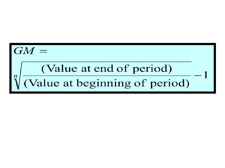
Other measures of Location • Geometric Mean of a set of n numbers is defined as the nth root of the product of the n numbers. • GM is used to average percentages, indexes, and relatives

Example 1 The interest rate on three bonds were 5, 21, and 4 percent. The arithmetic mean is (5+21+4) / 3 =10. 0 The geometric mean is The GM gives a more conservative profit figure because it is not heavily weighted by the rate of 21%

Example 2 Another use of GM is to determine the percent increase in sales, production or other business or economic series from one time period to another.

Example 3 The total number of females enrolled in American colleges increased from 755, 000 in 1992 to 835, 000 in 2000. That is, the geometric mean rate of increase is 1. 27%.

Measures of Dispersion • Range • Mean Deviation • Quartile Deviation • Standard Deviation • Variance • Co-efficient of Variation

Dispersion refers to the spread or variability in the data. mean Range = Largest value – Smallest value

Range Example The following represents the current year’s Return on Equity of the 25 companies in an investor’s portfolio. Highest value: 22. 1 Lowest value: -8. 1 Range = Highest value – lowest value = 22. 1 -(-8. 1) = 30. 2

Mean Deviation The arithmetic mean of the absolute values of the deviations from the arithmetic mean. [notation AD or MAD] m All values are used in the calculation. m It is not unduly influenced by large or small values. m The absolute values are difficult to manipulate.

AD or MAD for Grouped Data

Example 5 The weights of a sample of crates containing books for the bookstore (in pounds ) are: 103, 97, 101, 106, 103 X = 102

Standard deviation and Variance the arithmetic mean of the squared deviations from the mean Standard deviation = (variance) Population Variance X is the value of an observation in the population μ is the arithmetic mean of the population N is the number of observations in the population Population Standard Deviation, s

Example 6 In Example 4, the variance and standard deviation are: Sample variance Sample standard deviation, s

Example 7 The hourly wages earned by a sample of five students are $7, $5, $11, $8, $6.

Variance for Raw data and Grouped Data

Empirical Rule: For any symmetrical, bellshaped distribution 1. 2. 3. About 68% of the observations will lie within 1 s the mean About 95% of the observations will lie within 2 s of the mean Nearly all the observations will be within 3 s of the mean

Interpretation and Uses of the Standard Deviation 68% 95% 99. 7% m-3 s m-2 s m-1 s m m+1 s m+2 s m+ 3 s

Quartiles 25% Q 1, Q 2, Q 3 divides ranked data into four equal parts 25% Q 2 Q 1 25% Q 3 Fra 10 Deciles: D 1, D 2, D 3, D 4, D 5, D 6, D 7, D 8, D 9 divides ranked data into ten equal parts 10% 10% D 1 D 2 D 3 10% 10% D 4 D 5 cti les 10% 10% D 6 D 7 D 8 D 9 99 Percentiles: divides ranked data into 100 equal parts

Relative Standing • Percentile: percentile of value x = {((number of values < x)/ total number of values)}*100; [round the result to the nearest whole number] • Suppose that in a class of 25 people we have the following averages (ordered in ascending order • 42, 59, 63, 67, 69, 70, 73, 74, 74, 77, 78, 79, 80, 81, 84, 85, 87, 89, 91, 94, 98 • If you received a 77, what percentile are you? • percentile of 77 = (12/25)*100 = 48

Relative Standing- Quartiles • Instead of finding the percentile of a single data value as we did on the previous page, it is often useful to group the data into 4, or more, (nearly) equal groups. When grouping the data into four equal groupings, we call these groupings quartiles. • Let n = Sample Size; k = percent desired (ex. k= 25) and L = locator the value separating the first k percent of the data from the rest • L = (k/100) * n

• Let’s separate the 25 class grades into four quartiles • Step 1 – order the data in ascending order; 42, 59, 63, 67, 69, 70, 73, 74, 74, 77, 78, 79, 80, 81, 84, 85, 87, 89, 91, 94, 98 • Step 2 - find the 3 locators L 25, L 50, L 75 • L 25 = (25/100) * 25 = 6. 25 (6 th ) • L 50 = (50/100) * 25 = 12. 5 (13 th ) • L 75 = (75/100) * 25 = 18. 75 (19 th) • Round up to nature of data; Q 1=70; Q 2=77; Q 3=84

Relative Standing Other measures of relative standing include • Interquartile range (IQR) = Q 3 - Q 1 • Semi-interquartile range = (Q 3 Q 1)/ 2 • Midquartile = (Q 3 + Q 1)/2 • 10 – 90 percentile range = P 90 - P 10

Using data on Slide No. * • IQR = 84 – 70 = 16 • Semi IQR = (84 – 70)/2 = 8 • Midquartile = (84 + 70)/2 = 77

Percentile of score AX = number of scores less than AX total number of scores Relation between the different fractiles • Q 1 = P 25 • Q 2 = P 50 • Q 3 = P 75 Interquartile Range: Q 3 – Q 1 D 1 = P 10 D 2 = P 20 D 3 = P 30 • • • D 9 = P 90 * 100

Box Diagram L 25 65, 67, 68, 69, 71, 71, 72, 72, 73, 73, 74, 75, 75, 76, 77, 77, 77, 78, 78, 79, 79, 80, 81, 81, 82, 83, 84, 85, 85, 86, 87, 88, 89, 92 media n L 75 To construct a box diagram to illustrate the extent to which the extreme data values lie beyond the interquartile range, draw a line with the low and high value highlighted at the two ends. Mark the gradations between these two extremes, then locate the quartile boundaries Q 1, Med. , and Q 3 on this line. Construct a box about Q 1 = (73 + 74)/2 = 73. 5 these values. Q 1 Q 3 65 69 89 73 M 77 81 85 92

Box plot graphical display, based on quartiles, that helps to picture a set of data. Five pieces of data are needed to construct a box plot: Minimum Value, First Quartile, Q 1 Median, Third Quartile, Q 3 Maximum Value. The box represents the interquartile range which contains the 50% of values. The whiskers represent the range; they extend from the box to the highest and lowest values, excluding outliers. A line across the box indicates the median.

Example 8 Based on a sample of 20 deliveries, Buddy’s Pizza determined the following information. The minimum delivery time was 13 minutes and the maximum 30 minutes. The first quartile was 15 minutes, the median 18 minutes, and the third quartile 22 minutes. Develop a box plot for the delivery times. 1. 5 times the IQ range 1. 5 times the interquartile range

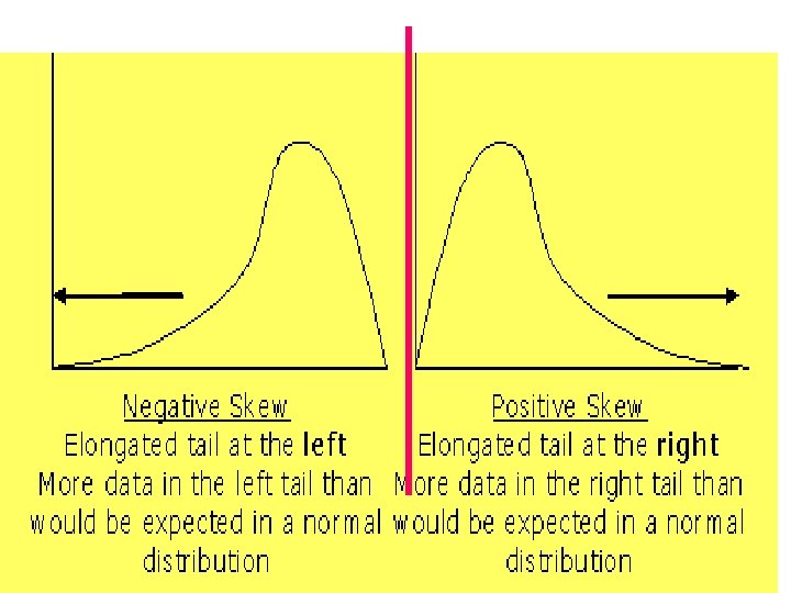
Skewness- measurement of the lack of symmetry of a distribution • Symmetric distribution: A distribution having the same shape on either side of the centre • Skewed distribution: One whose shapes on either side of the center differ; a nonsymmetrical distribution • A distribution can be positively or negatively skewed

Relative Positions of the Mean, Median, and Mode in a Symmetric Distribution

Relative Positions of the Mean, Median, and Mode in a Right Skewed or Positively Skewed Distribution Mean > Median > Mode

The Relative Positions of the Mean, Median, and Mode in a Left Skewed or Negatively Skewed Distribution Mean < Median < Mode

SKEWNESS

The coefficient of skewness can range from 3. 00 up to 3. 00 A value of 0 indicates a symmetric distribution. Example 9 Using the twelve stock prices, we find the mean to be 84. 42, standard deviation, 7. 18, median, 84. 5. = -0. 03

SKEWNESS FOR GROUPED DATA

Kurtosis derived from the Greek word κυρτός, kyrtos or kurtos, meaning bulging • • measure of the "peakedness" of the probability distribution of a real-valued random variable • higher kurtosis means more of the variance is due to infrequent extreme deviations, as opposed to frequent modestly-sized deviations.

distribution with positive kurtosis is called leptokurtic, or leptokurtotic. In terms of shape, a leptokurtic distribution has a more acute "peak" around the mean (that is, a higher probability than a normally distributed variable of values near the mean) and "fat tails" (that is, a higher probability than a normally distributed variable of extreme values). distribution with negative kurtosis is called platykurtic, or platykurtotic. In terms of shape, a platykurtic distribution has a smaller "peak" around the mean (that is, a lower probability than a normally distributed variable of values near the mean) and "thin tails" (that is, a lower probability than a normally distributed variable of extreme values).

Other distribution – Leptokurtic Normal distribution - Mesokurtic Other distribution – Platykurtic

Comparing Standard Deviations Data A 11 12 13 14 15 16 17 18 19 20 21 Mean = 15. 5 s = 3. 338 Data B 11 12 13 14 15 16 17 18 19 20 21 Mean = 15. 5 s =. 9258 Data C 11 12 13 14 15 16 17 18 19 20 21 Mean = 15. 5 s = 4. 57

Co-efficient of variation • Measures relative variation • Always in percentage (%) • Shows variation relative to mean • Is used to compare two or more sets of data measured in different units When the mean value is near zero, the coefficient of variation is sensitive to change in the standard deviation, limiting its usefulness.

Stock A: Average price last year = $50 Standard deviation = $5 Stock B: Average price last year = $100 Standard deviation = $5

• Next Lecture Is On Probability – Revise Your Knowledge Of Sets