Wrapup of Econ 1 Today A summary of

Wrap-up of Econ 1 Today: A summary of marginal analysis and equilibrium; a review of the 16 chapters

Wrapping up this class n Today’s lecture is meant to do two things n n Highlight some material you will need to know for the final exam Help put all of the ideas together so that you can use the ideas in this class in future classes and the real world

Marginal analysis n n n Marginal analysis is almost always important Average analysis is important sometimes Recall the following slide from the first lecture…

What will we do in Econ 1? n Think like an economist does n n n (Almost) always think in terms of marginal Opportunity costs typically matter Sunk costs typically do not matter n Marginal “one additional unit” n For example, FB describe marginal benefit as “the increase in total benefit that results from carrying out one additional unit of an activity” (p. 11)

Marginal analysis n n Marginal analysis will continue to be important if you plan on majoring in anything with economics as a tool When faced with problems in the real world, try to think marginally with the tools we have learned

Marginal analysis n n n In most markets, a firm or consumer will continue an activity as long as its MB ≥ MC Without market failure, equilibrium is efficient Market failures with market power and/or externalities n Situations exist where government intervention improves efficiency

Marginal analysis n Finally, marginal analysis applies to various topics we have discussed in recent weeks n n n Information Labor markets Quality of life issues Public Goods Tax Policy

What have we covered the past 9+ weeks? n n 16 chapters that give you a foundation of microeconomics Let’s highlight each chapter

Chapter 1: Think like an economist n n n Usually avoid averages in analysis Don’t ignore opportunity cost Don’t ignore sunk costs Think marginally Try to find Pareto improvements when possible

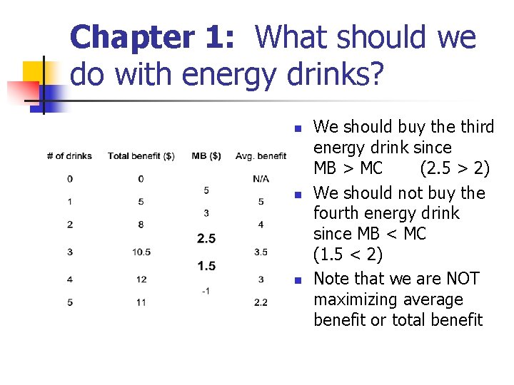
Chapter 1: What should we do with energy drinks? n n n We should buy the third energy drink since MB > MC (2. 5 > 2) We should not buy the fourth energy drink since MB < MC (1. 5 < 2) Note that we are NOT maximizing average benefit or total benefit

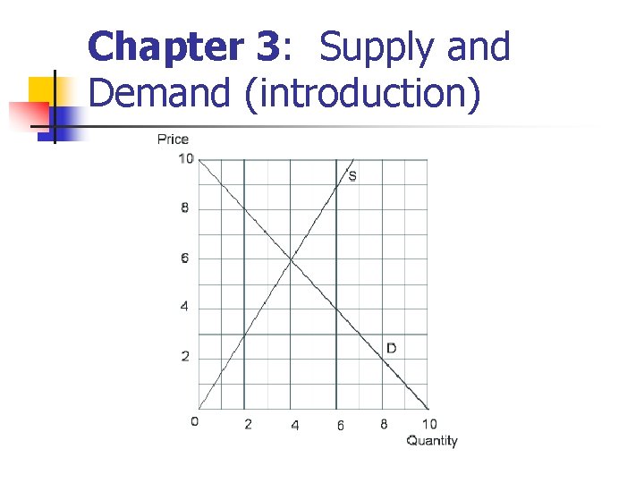
Chapter 3: Supply and Demand (introduction)

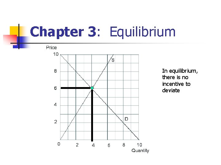
Chapter 3: Equilibrium In equilibrium, there is no incentive to deviate

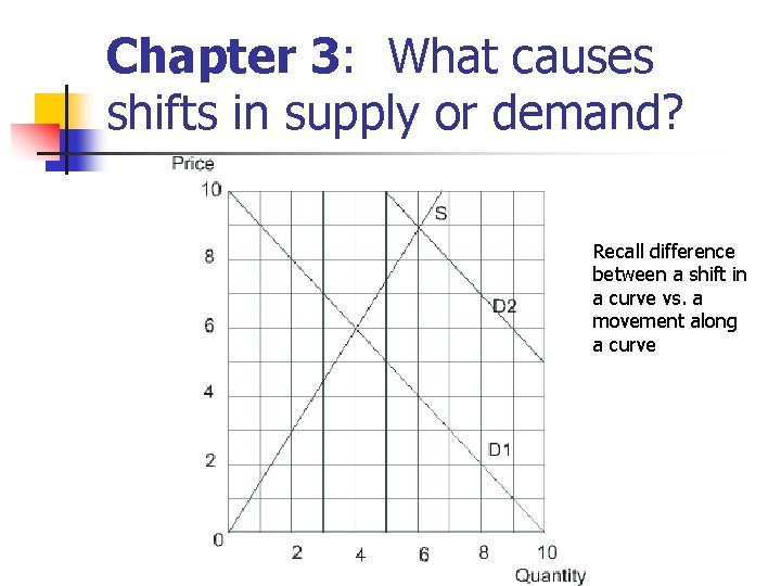
Chapter 3: What causes shifts in supply or demand? Recall difference between a shift in a curve vs. a movement along a curve

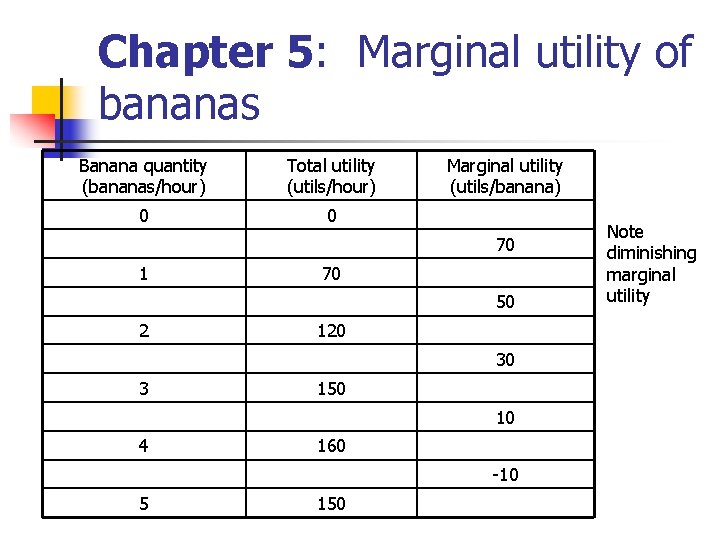
Chapter 5: Marginal utility of bananas Banana quantity (bananas/hour) Total utility (utils/hour) 0 0 Marginal utility (utils/banana) 70 1 70 50 2 120 30 3 150 10 4 160 -10 5 150 Note diminishing marginal utility

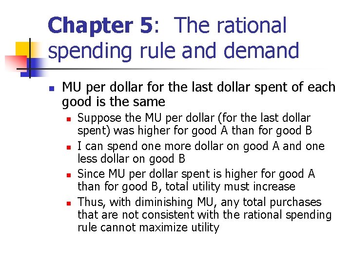
Chapter 5: The rational spending rule and demand n MU per dollar for the last dollar spent of each good is the same n n Suppose the MU per dollar (for the last dollar spent) was higher for good A than for good B I can spend one more dollar on good A and one less dollar on good B Since MU per dollar spent is higher for good A than for good B, total utility must increase Thus, with diminishing MU, any total purchases that are not consistent with the rational spending rule cannot maximize utility

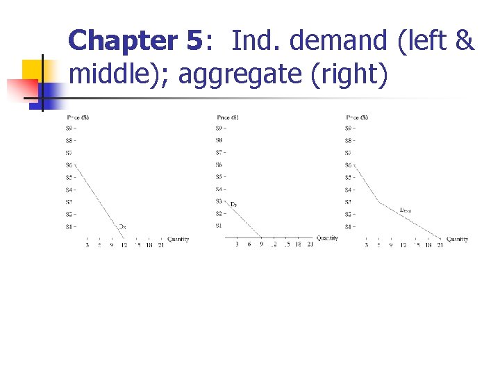
Chapter 5: Ind. demand (left & middle); aggregate (right)

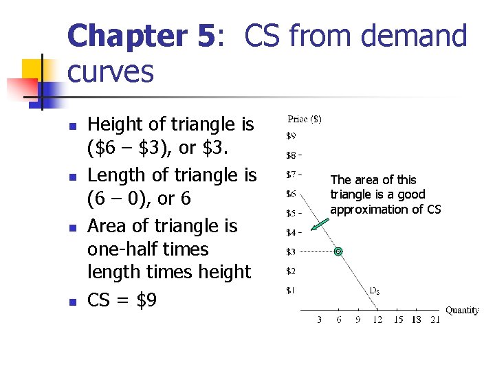
Chapter 5: CS from demand curves n n Height of triangle is ($6 – $3), or $3. Length of triangle is (6 – 0), or 6 Area of triangle is one-half times length times height CS = $9 The area of this triangle is a good approximation of CS

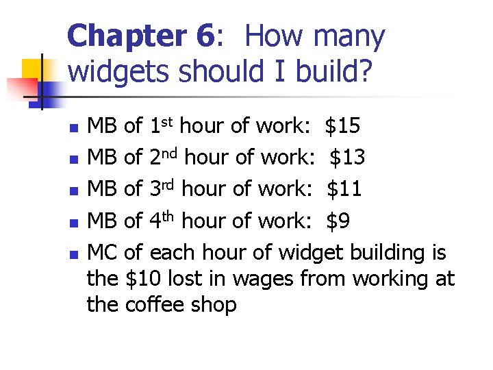
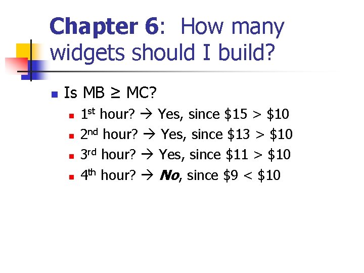
Chapter 6: How many widgets should I build? n n n MB of 1 st hour of work: $15 MB of 2 nd hour of work: $13 MB of 3 rd hour of work: $11 MB of 4 th hour of work: $9 MC of each hour of widget building is the $10 lost in wages from working at the coffee shop

Chapter 6: How many widgets should I build? n Is MB ≥ MC? n n 1 st hour? Yes, since $15 > $10 2 nd hour? Yes, since $13 > $10 3 rd hour? Yes, since $11 > $10 4 th hour? No, since $9 < $10

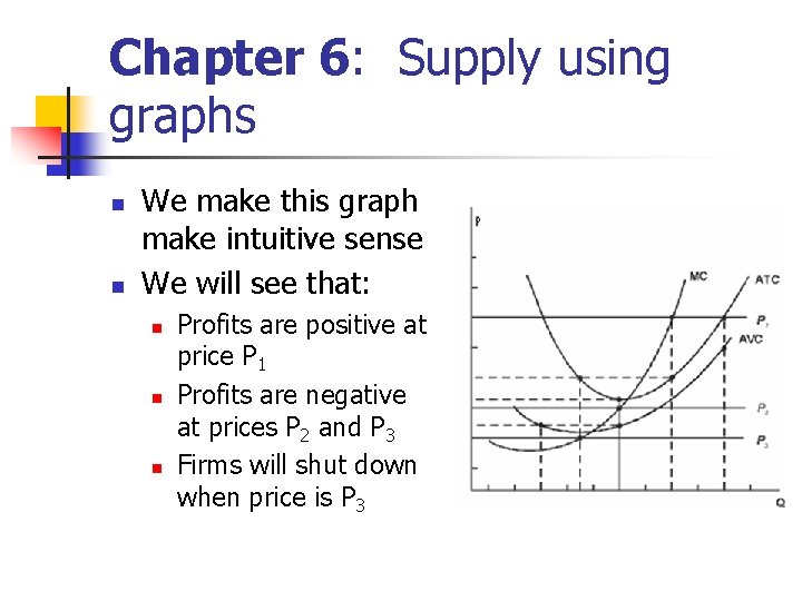
Chapter 6: Supply using graphs n n We make this graph make intuitive sense We will see that: n n n Profits are positive at price P 1 Profits are negative at prices P 2 and P 3 Firms will shut down when price is P 3

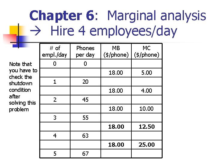
Chapter 6: Marginal analysis Hire 4 employees/day Note that you have to check the shutdown condition after solving this problem # of empl. /day Phones per day 0 0 1 2 3 4 5 MB MC ($/phone) 18. 00 5. 00 18. 00 4. 00 18. 00 10. 00 18. 00 12. 50 18. 00 25. 00 20 45 55 63 67

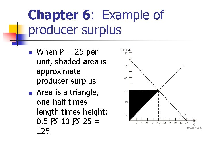
Chapter 6: Example of producer surplus n n When P = 25 per unit, shaded area is approximate producer surplus Area is a triangle, one-half times length times height: 0. 5 10 25 = 125

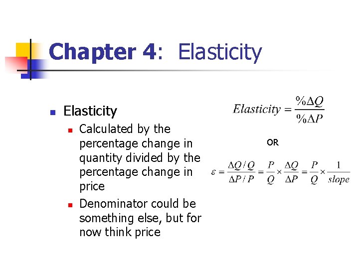
Chapter 4: Elasticity n n Calculated by the percentage change in quantity divided by the percentage change in price Denominator could be something else, but for now think price OR

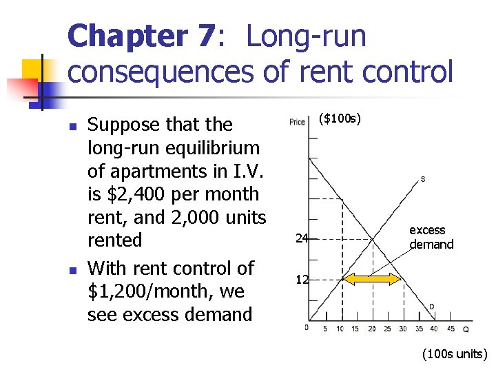
Chapter 7: Long-run consequences of rent control n n Suppose that the long-run equilibrium of apartments in I. V. is $2, 400 per month rent, and 2, 000 units rented With rent control of $1, 200/month, we see excess demand ($100 s) 24 excess demand 12 (100 s units)

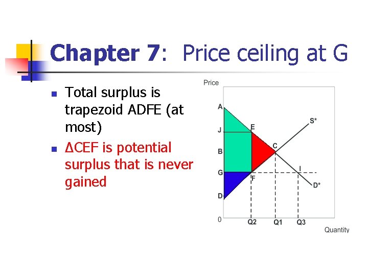
Chapter 7: Price ceiling at G n n Total surplus is trapezoid ADFE (at most) ΔCEF is potential surplus that is never gained

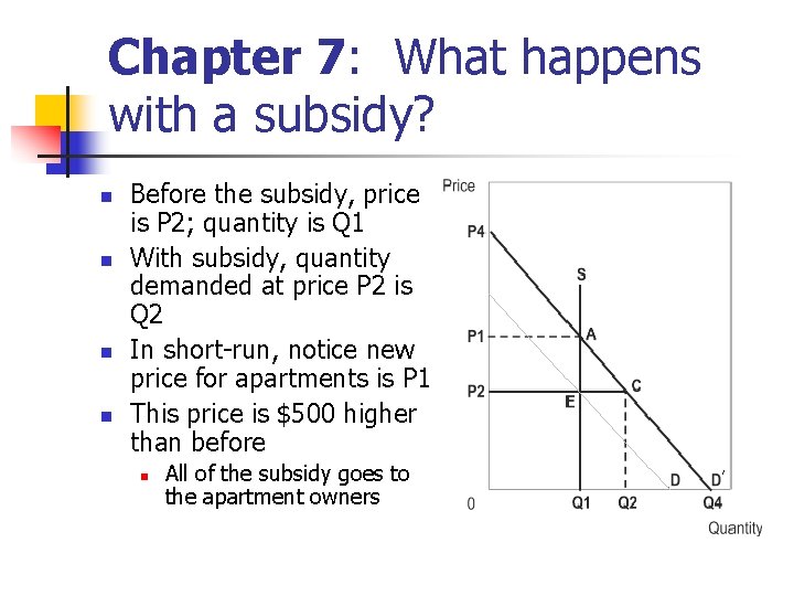
Chapter 7: What happens with a subsidy? n n Before the subsidy, price is P 2; quantity is Q 1 With subsidy, quantity demanded at price P 2 is Q 2 In short-run, notice new price for apartments is P 1 This price is $500 higher than before n All of the subsidy goes to the apartment owners

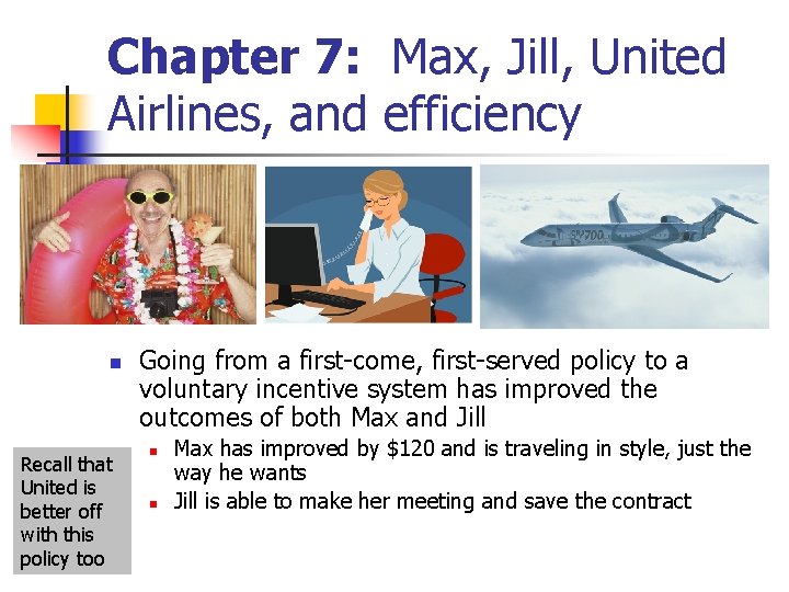
Chapter 7: Max, Jill, United Airlines, and efficiency n Recall that United is better off with this policy too Going from a first-come, first-served policy to a voluntary incentive system has improved the outcomes of both Max and Jill n n Max has improved by $120 and is traveling in style, just the way he wants Jill is able to make her meeting and save the contract

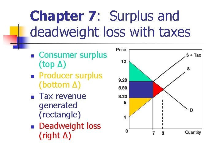
Chapter 7: Surplus and deadweight loss with taxes n n Consumer surplus (top Δ) Producer surplus (bottom Δ) Tax revenue generated (rectangle) Deadweight loss (right Δ)

Chapter 7: Marginal cost pricing n Supply of electricity n n 8 Mwh (coal) @ 3¢/Kwh 20 Mwh (natural gas) @ 5¢/Kwh 10 Mwh (wind power) @ 9¢/Kwh 6 Mwh (solar power) @ 15¢/Kwh n n n Suppose that at a price of 9¢/Kwh, 30 Mwh were demanded All coal capacity and natural gas capacity can be used, and 2 Mwh provided by wind MC pricing tells us to charge 9 ¢/Kwh in order to maximize surplus

Chapter 8: What should Jill do? n n n Jill should run a home business if her economic profit is positive Economic profit is total revenue minus all costs (including opportunity cost of not working) Economic profit if she opens business = $200, 000 – ($160, 000 + $60, 000) = – $20, 000 Do not open business

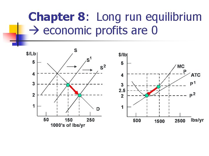
Chapter 8: Long run equilibrium economic profits are 0

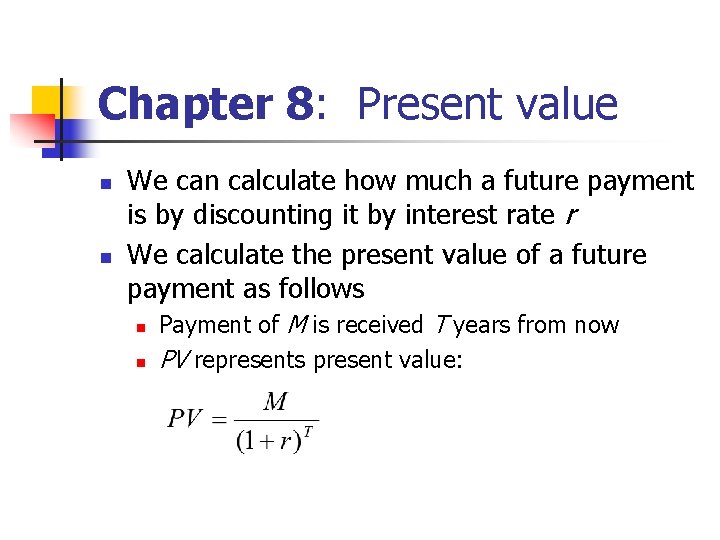
Chapter 8: Present value n n We can calculate how much a future payment is by discounting it by interest rate r We calculate the present value of a future payment as follows n n Payment of M is received T years from now PV represents present value:

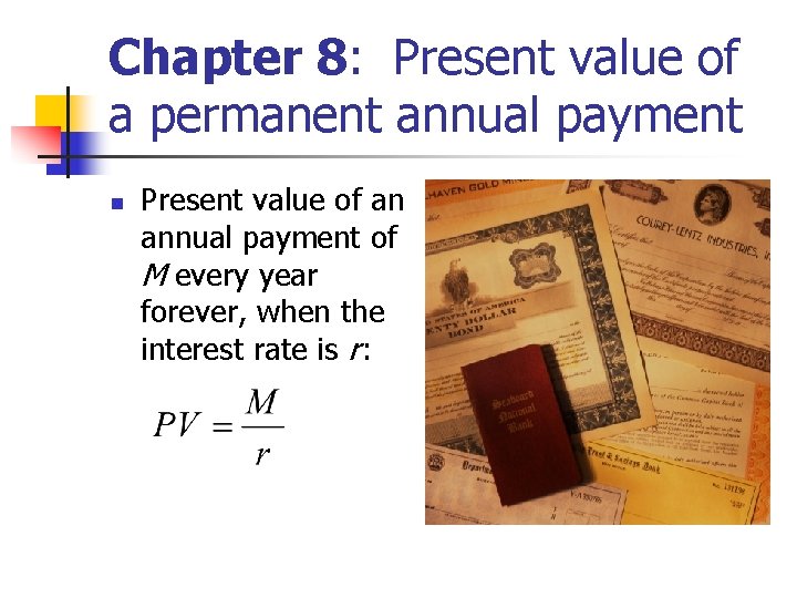
Chapter 8: Present value of a permanent annual payment n Present value of an annual payment of M every year forever, when the interest rate is r :

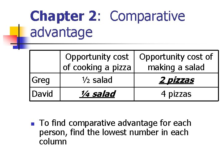
Chapter 2: Absolute advantage and comparative advantage n Absolute advantage n n “One person has an absolute advantage over another if he or she takes fewer hours to perform a task than the other person” (F/B p. 36) Comparative advantage n “One person has a comparative advantage over another if his or her opportunity cost of performing a task is lower than the other person’s opportunity cost” (F/B p. 37)

Chapter 2: Comparative advantage Greg David n Opportunity cost of of cooking a pizza making a salad ½ salad 2 pizzas ¼ salad 4 pizzas To find comparative advantage for each person, find the lowest number in each column

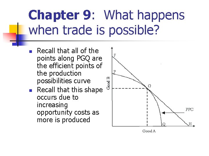
Chapter 9: What happens when trade is possible? n n Recall that all of the points along PGQ are the efficient points of the production possibilities curve Recall that this shape occurs due to increasing opportunity costs as more is produced

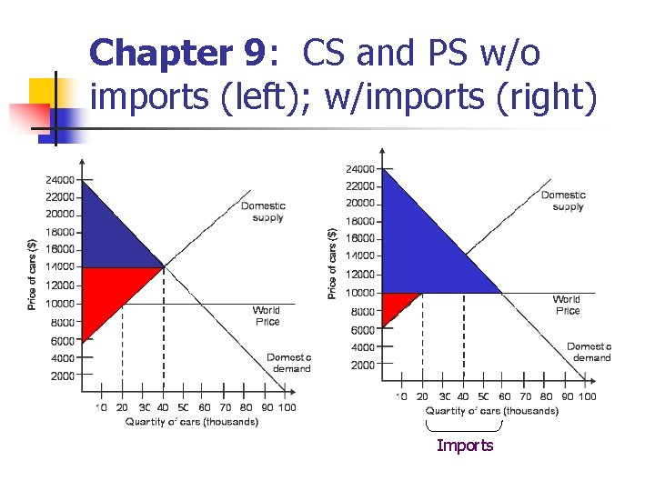
Chapter 9: CS and PS w/o imports (left); w/imports (right) Imports

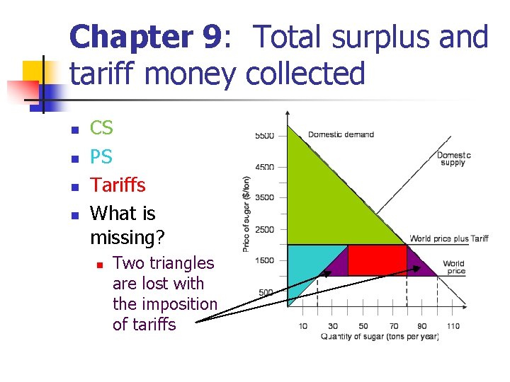
Chapter 9: Total surplus and tariff money collected n n CS PS Tariffs What is missing? n Two triangles are lost with the imposition of tariffs

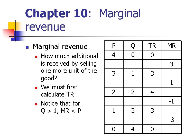
Chapter 10: Marginal revenue n n n How much additional is received by selling one more unit of the good? We must first calculate TR Notice that for Q > 1, MR < P P 4 Q 0 TR 0 MR 3 3 1 2 2 4 -1 1 3 3 -3 0 4 0

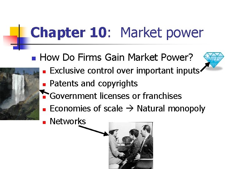
Chapter 10: Market power n How Do Firms Gain Market Power? n n n Exclusive control over important inputs Patents and copyrights Government licenses or franchises Economies of scale Natural monopoly Networks

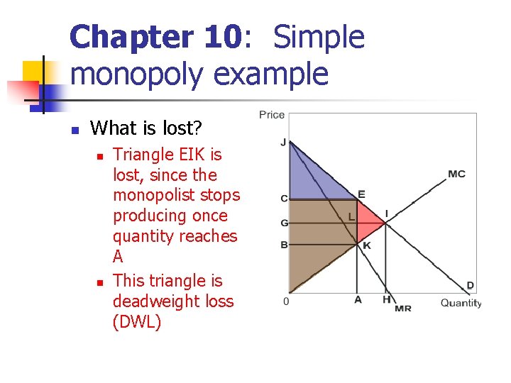
Chapter 10: Simple monopoly example n What is lost? n n Triangle EIK is lost, since the monopolist stops producing once quantity reaches A This triangle is deadweight loss (DWL)

Chapter 10: Price discrimination n Price discrimination can take many forms n n n Discounts of goods and services that have little or no value if transferred to another person Perfect price discrimination, where a different price can be charged to each person Rebates, which require effort to get a discount

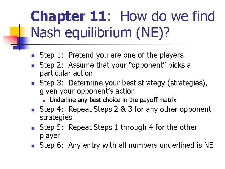
Chapter 11: How do we find Nash equilibrium (NE)? n n n Step 1: Pretend you are one of the players Step 2: Assume that your “opponent” picks a particular action Step 3: Determine your best strategy (strategies), given your opponent’s action n n Underline any best choice in the payoff matrix Step 4: Repeat Steps 2 & 3 for any other opponent strategies Step 5: Repeat Steps 1 through 4 for the other player Step 6: Any entry with all numbers underlined is NE

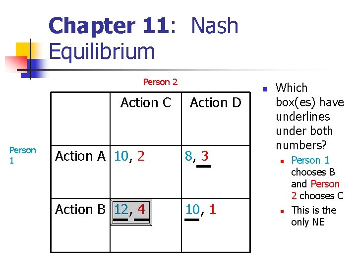
Chapter 11: Nash Equilibrium Person 2 Action C Person 1 Action D Action A 10, 2 8, 3 Action B 12, 4 10, 1 n Which box(es) have underlines under both numbers? n n Person 1 chooses B and Person 2 chooses C This is the only NE

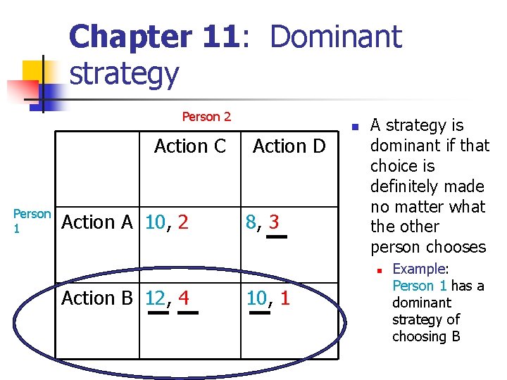
Chapter 11: Dominant strategy Person 2 Action C Person 1 Action A 10, 2 Action D 8, 3 n A strategy is dominant if that choice is definitely made no matter what the other person chooses n Action B 12, 4 10, 1 Example: Person 1 has a dominant strategy of choosing B

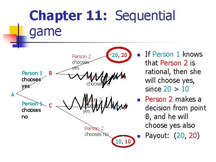
Chapter 11: Sequential game Person 1 B chooses yes A Person 1 C chooses no Person 2 chooses yes 20, 20 n Person 2 5, 10 chooses no Person 2 chooses yes n 10, 5 Person 2 chooses no 10, 10 n If Person 1 knows that Person 2 is rational, then she will choose yes, since 20 > 10 Person 2 makes a decision from point B, and he will choose yes also Payout: (20, 20)

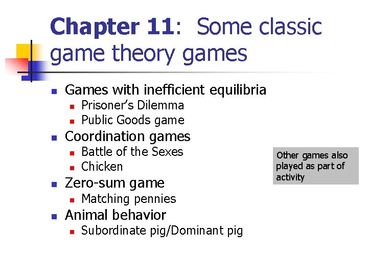
Chapter 11: Some classic game theory games n Games with inefficient equilibria n n n Coordination games n n n Battle of the Sexes Chicken Zero-sum game n n Prisoner’s Dilemma Public Goods game Matching pennies Animal behavior n Subordinate pig/Dominant pig Other games also played as part of activity

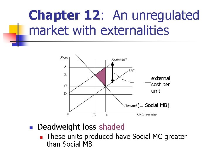
Chapter 12: An unregulated market with externalities external cost per unit (= Social MB) n Deadweight loss shaded n These units produced have Social MC greater than Social MB

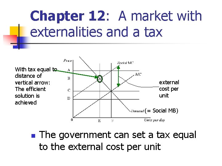
Chapter 12: A market with externalities and a tax With tax equal to distance of vertical arrow: The efficient solution is achieved external cost per unit (= Social MB) n The government can set a tax equal to the external cost per unit

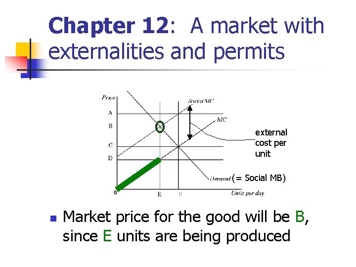
Chapter 12: A market with externalities and permits external cost per unit (= Social MB) n Market price for the good will be B, since E units are being produced

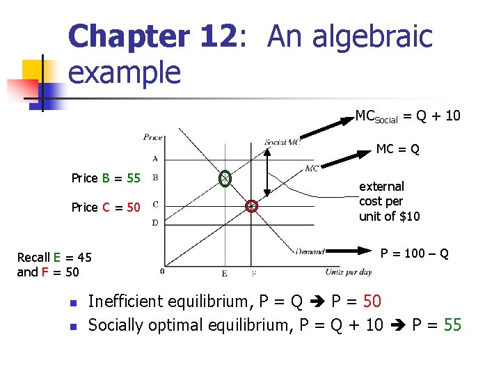
Chapter 12: An algebraic example MCSocial = Q + 10 MC = Q Price B = 55 Price C = 50 Recall E = 45 and F = 50 n n external cost per unit of $10 P = 100 – Q Inefficient equilibrium, P = Q P = 50 Socially optimal equilibrium, P = Q + 10 P = 55

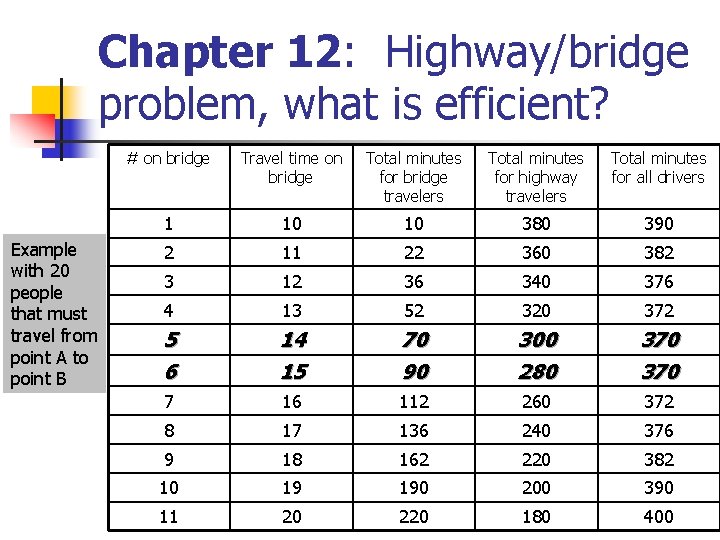
Chapter 12: Highway/bridge problem, what is efficient? Example with 20 people that must travel from point A to point B # on bridge Travel time on bridge Total minutes for bridge travelers Total minutes for highway travelers Total minutes for all drivers 1 10 10 380 390 2 11 22 360 382 3 12 36 340 376 4 13 52 320 372 5 6 14 15 70 90 300 280 370 7 16 112 260 372 8 17 136 240 376 9 18 162 220 382 10 19 190 200 390 11 20 220 180 400

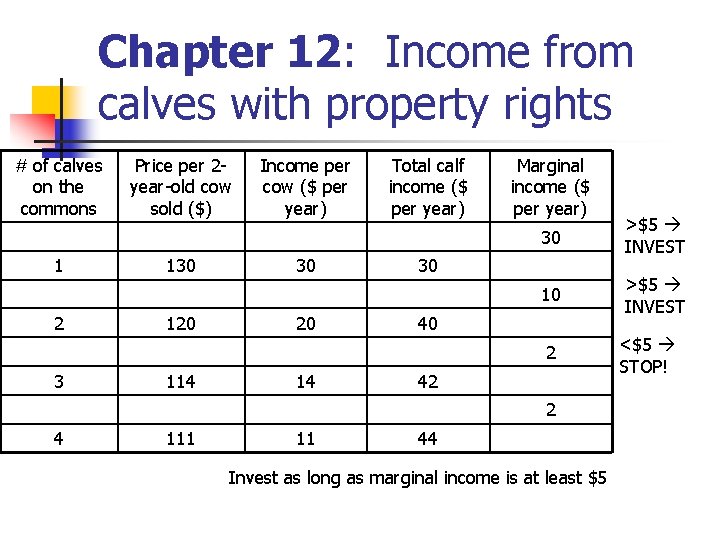
Chapter 12: Income from calves with property rights # of calves on the commons Price per 2 year-old cow sold ($) Income per cow ($ per year) Total calf income ($ per year) Marginal income ($ per year) 30 1 130 30 30 10 2 120 20 40 2 3 114 14 42 2 4 111 11 44 Invest as long as marginal income is at least $5 >$5 INVEST <$5 STOP!

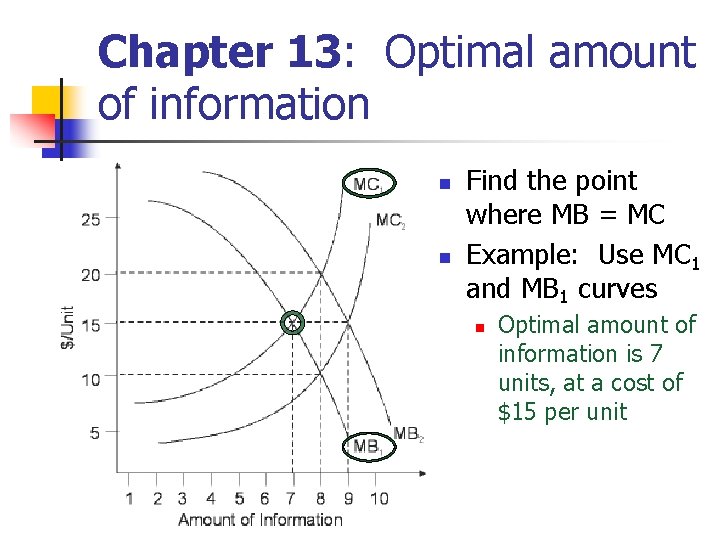
Chapter 13: Optimal amount of information n n Find the point where MB = MC Example: Use MC 1 and MB 1 curves n Optimal amount of information is 7 units, at a cost of $15 per unit

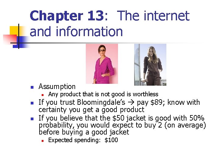
Chapter 13: The internet and information n Assumption n Any product that is not good is worthless If you trust Bloomingdale’s pay $89; know with certainty you get a good product If you believe that the $50 jacket is good with 50% probability, you would expect to buy 2 (on average) before buying a good jacket n Expected spending: $100

Yugo car Chapter 13: Lemons n A used car dealer has the following information about used Yugo limos: n Plums are worth n n n Lemons are worth n n n $3, 000 to the dealer $1, 200 to the owner $250 to the dealer $100 to the owner 100 Yugo limos owned privately n n Example 1: Half of the limos are plums, half are lemons Example 2: One-quarter of the limos are plums, threequarters are lemons

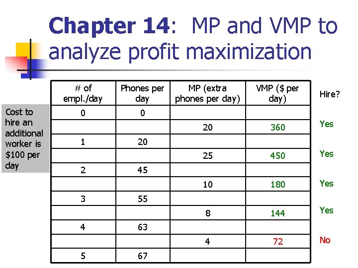
Chapter 14: MP and VMP to analyze profit maximization # of empl. /day Cost to hire an additional worker is $100 per day 0 1 2 3 4 5 Phones per MP (extra day phones per day) VMP ($ per day) 0 Hire? 20 360 Yes 25 450 Yes 10 180 Yes 8 144 Yes 4 72 No 20 45 55 63 67

Chapter 14: Some human capital qualities n Education n n Direct knowledge Intelligence Signaling Training Work and life experiences n n Energy level Work habits Trustworthiness Initiative

Chapter 14: When are unions effective? n Finding qualified workers outside of a union is difficult or impossible n Example: Writers’ strike n n n See “Additional reading” on class website for more on this topic When a firm is making economic profits When a unionized firm can hire better workers than nonunionized firms

Chapter 14: Discrimination n A wage gap between men and women’s pay has existed for decades n n Some of this can be explained by controlling for education, experience, and other factors Some discrimination may be occurring n Firms that do discriminate based on factors such as gender and race are less likely to be competitive in the long run

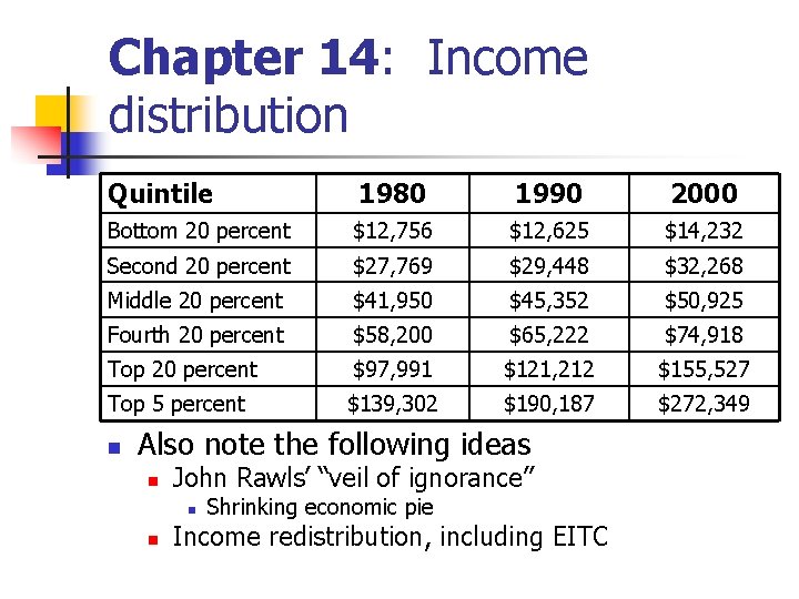
Chapter 14: Income distribution Quintile 1980 1990 2000 Bottom 20 percent $12, 756 $12, 625 $14, 232 Second 20 percent $27, 769 $29, 448 $32, 268 Middle 20 percent $41, 950 $45, 352 $50, 925 Fourth 20 percent $58, 200 $65, 222 $74, 918 Top 20 percent $97, 991 $121, 212 $155, 527 Top 5 percent $139, 302 $190, 187 $272, 349 n Also note the following ideas n John Rawls’ “veil of ignorance” n n Shrinking economic pie Income redistribution, including EITC

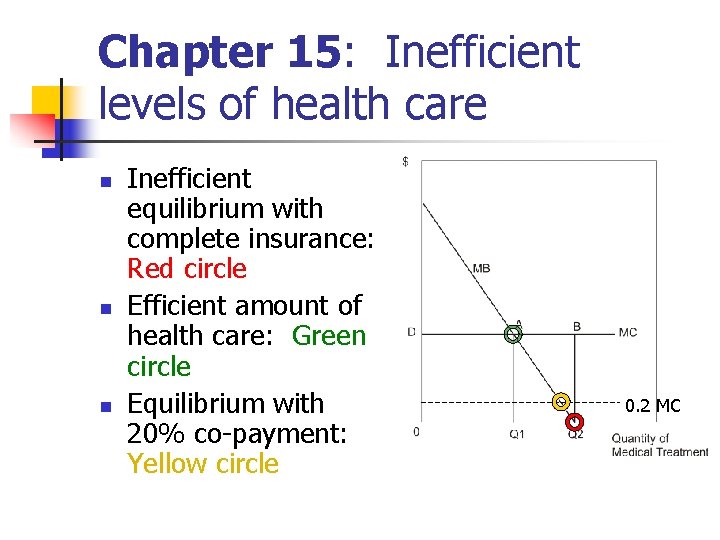
Chapter 15: Inefficient levels of health care n n n Inefficient equilibrium with complete insurance: Red circle Efficient amount of health care: Green circle Equilibrium with 20% co-payment: Yellow circle 0. 2 MC

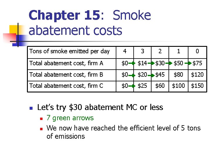
Chapter 15: Smoke abatement costs Tons of smoke emitted per day 4 3 2 1 0 Total abatement cost, firm A $0 $14 $30 $50 $75 Total abatement cost, firm B $0 $20 $45 $80 $120 Total abatement cost, firm C $0 $25 $60 $100 $150 n Let’s try $30 abatement MC or less n n 7 green arrows We now have reached the efficient level of 5 tons of emissions

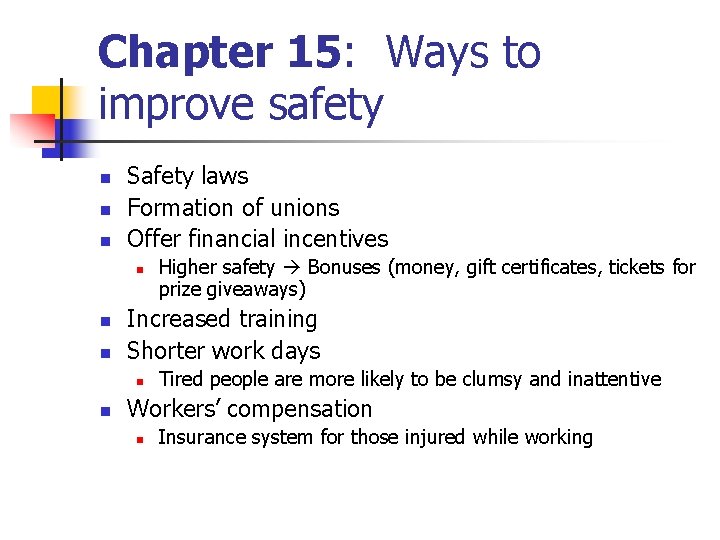
Chapter 15: Ways to improve safety n n n Safety laws Formation of unions Offer financial incentives n n n Increased training Shorter work days n n Higher safety Bonuses (money, gift certificates, tickets for prize giveaways) Tired people are more likely to be clumsy and inattentive Workers’ compensation n Insurance system for those injured while working

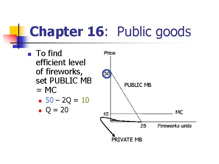
Chapter 16: Public goods n To find efficient level of fireworks, set PUBLIC MB = MC n n PUBLIC MB 50 – 2 Q = 10 Q = 20 MC PRIVATE MB

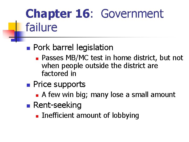
Chapter 16: Government failure n Pork barrel legislation n n Price supports n n Passes MB/MC test in home district, but not when people outside the district are factored in A few win big; many lose a small amount Rent-seeking n Inefficient amount of lobbying

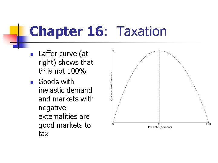
Chapter 16: Taxation n n Laffer curve (at right) shows that t* is not 100% Goods with inelastic demand markets with negative externalities are good markets to tax