Routing Games ECON 425563 CPSC 455555 9302008 1


- Slides: 48
Routing Games ECON 425/563 & CPSC 455/555 9/30/2008 1
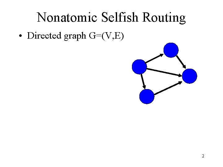
Nonatomic Selfish Routing • Directed graph G=(V, E) 2
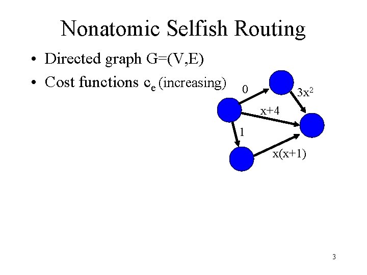
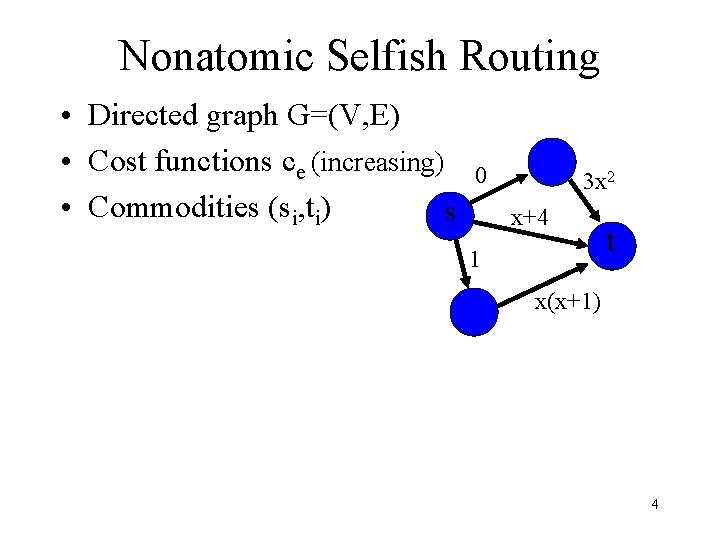
Nonatomic Selfish Routing • Directed graph G=(V, E) • Cost functions ce (increasing) 0 3 x 2 x+4 1 x(x+1) 3
Nonatomic Selfish Routing • Directed graph G=(V, E) • Cost functions ce (increasing) • Commodities (si, ti) s 0 3 x 2 x+4 1 t x(x+1) 4
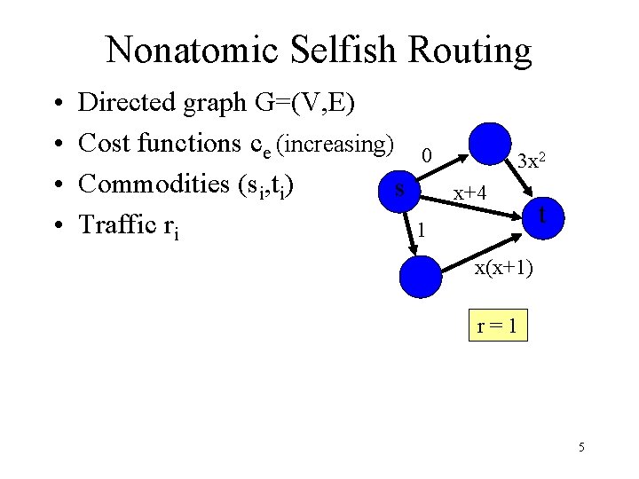
Nonatomic Selfish Routing • • Directed graph G=(V, E) Cost functions ce (increasing) Commodities (si, ti) s Traffic ri 0 3 x 2 x+4 1 t x(x+1) r=1 5
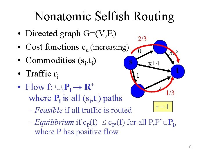
Nonatomic Selfish Routing • • • Directed graph G=(V, E) Cost functions ce (increasing) Commodities (si, ti) s Traffic ri Flow f: i. Pi R+ where Pi is all (si, ti) paths 2/3 0 3 x 2 x+4 t 1 x 1/3 r=1 – Feasible if all traffic is routed – Equilibrium if c. P(f) c. P’(f) for all P, P’ Pi, where P has positive flow 6
Nonatomic Selfish Routing • • • Directed graph G=(V, E) Cost functions ce (increasing) Commodities (si, ti) s Traffic ri Flow f: i. Pi R+ where Pi is all (si, ti) paths 2/3 0 3 x 2 x+4 t 1 x 1/3 r=1 – Feasible if all traffic is routed – Equilibrium if c. P(f) c. P’(f) for all si-ti paths P, P’ with positive flow • Social cost: c(f) = i P Pic. P(f) · f(P) 7
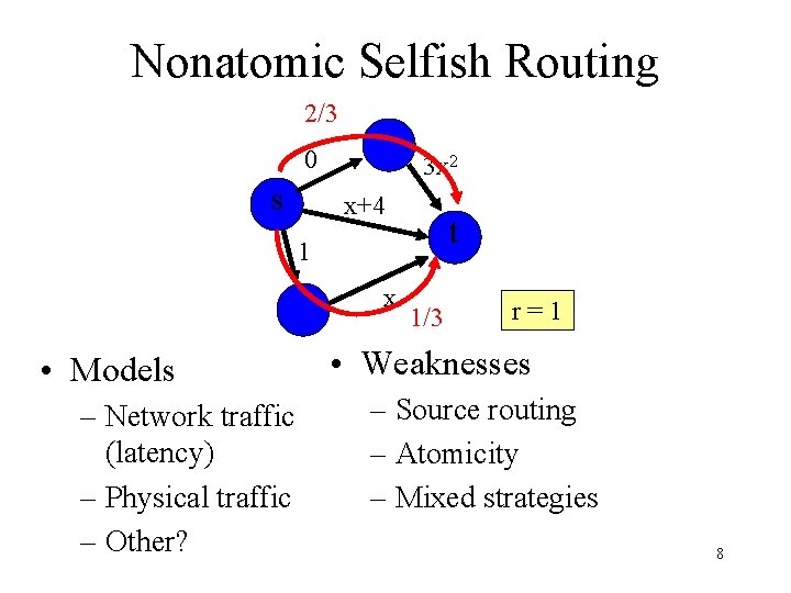
Nonatomic Selfish Routing 2/3 0 s 3 x 2 x+4 t 1 x • Models – Network traffic (latency) – Physical traffic – Other? 1/3 r=1 • Weaknesses – Source routing – Atomicity – Mixed strategies 8
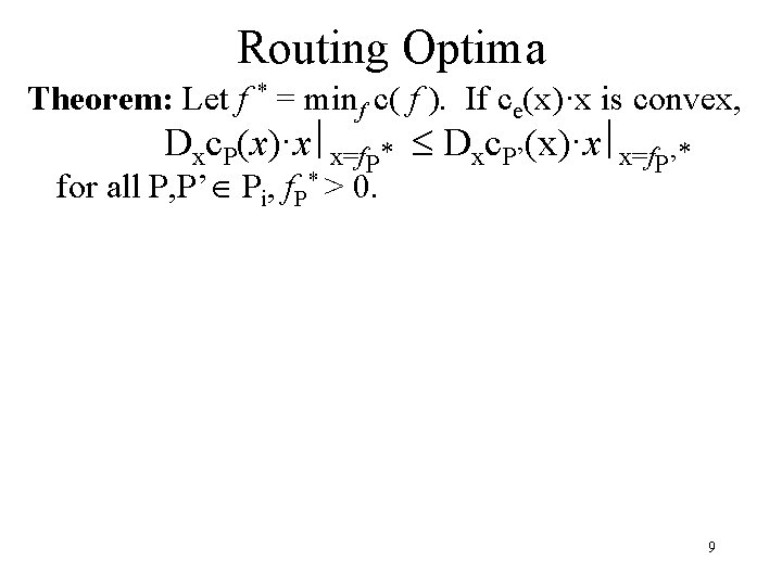
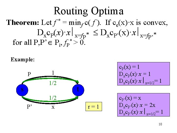
Routing Optima Theorem: Let f * = minf c( f ). If ce(x)·x is convex, Dxc. P(x)·x x=f. P* Dxc. P’(x)·x x=f. P’* for all P, P’ Pi, f. P* > 0. 9
Routing Optima Theorem: Let f * = minf c( f ). If ce(x)·x is convex, Dxc. P(x)·x x=f. P* Dxc. P’(x)·x x=f. P’* for all P, P’ Pi, f. P* > 0. Example: P 1 1/2 s P’ c. P(x) = 1 Dxc. P(x)·x x=1/2= 1 1/2 x t r=1 c. P’(x) = x Dxc. P’(x)·x = 2 x Dxc. P’(x)·x x=1/2= 1 10
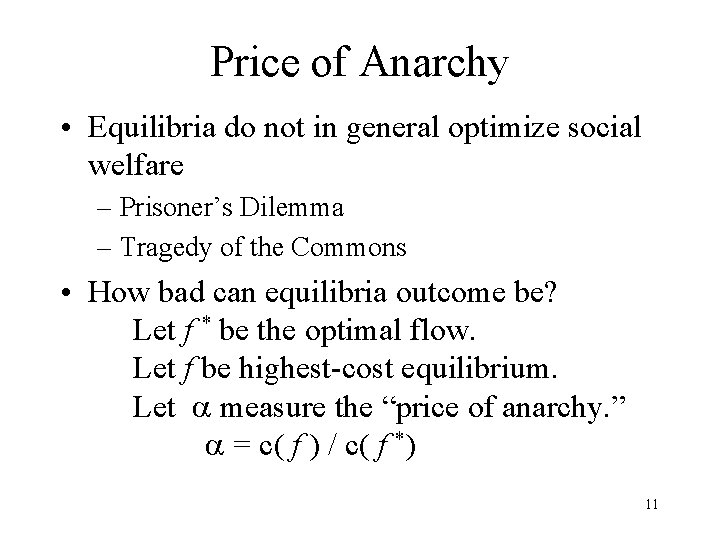
Price of Anarchy • Equilibria do not in general optimize social welfare – Prisoner’s Dilemma – Tragedy of the Commons • How bad can equilibria outcome be? Let f * be the optimal flow. Let f be highest-cost equilibrium. Let measure the “price of anarchy. ” = c( f ) / c( f *) 11
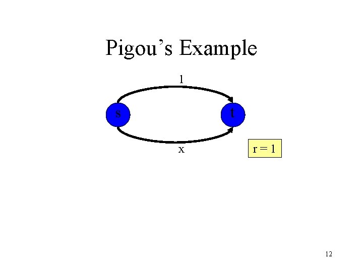
Pigou’s Example 1 s t x r=1 12
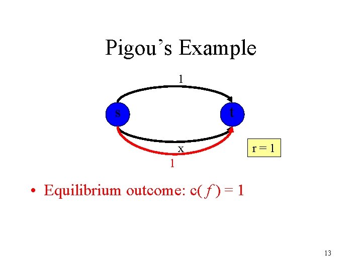
Pigou’s Example 1 s t x r=1 1 • Equilibrium outcome: c( f ) = 1 13
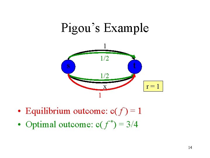
Pigou’s Example 1 s 1/2 t 1/2 x 1 r=1 • Equilibrium outcome: c( f ) = 1 • Optimal outcome: c( f *) = 3/4 14
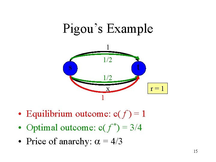
Pigou’s Example 1 s 1/2 t 1/2 x 1 r=1 • Equilibrium outcome: c( f ) = 1 • Optimal outcome: c( f *) = 3/4 • Price of anarchy: = 4/3 15
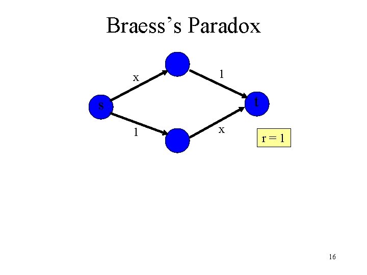
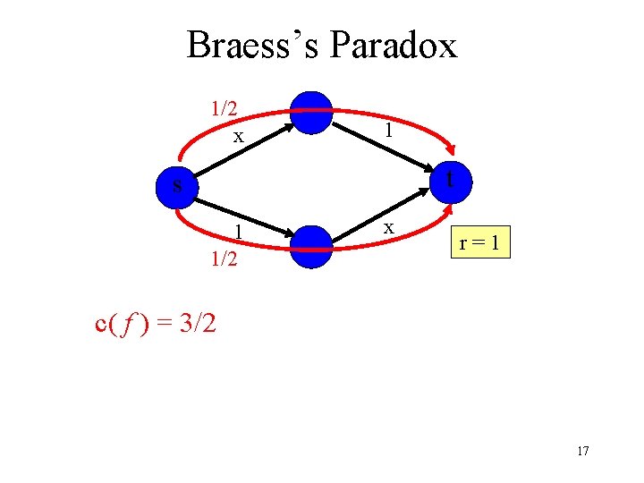
Braess’s Paradox x 1 t s 1 x r=1 16
Braess’s Paradox 1/2 x 1 t s 1 1/2 x r=1 c( f ) = 3/2 17
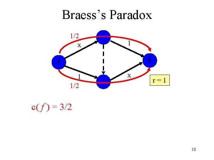
Braess’s Paradox 1/2 x 1 t s 1 1/2 x r=1 c( f ) = 3/2 18
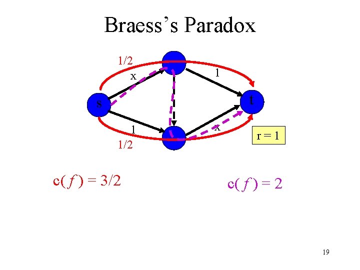
Braess’s Paradox 1/2 x 1 t s 1 1/2 c( f ) = 3/2 x r=1 c( f ) = 2 19
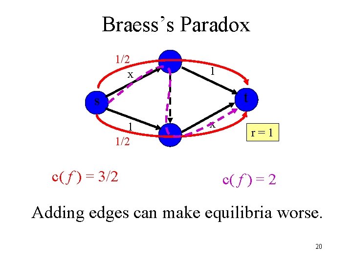
Braess’s Paradox 1/2 x 1 t s 1 1/2 c( f ) = 3/2 x r=1 c( f ) = 2 Adding edges can make equilibria worse. 20
Capacity Augmentation 21
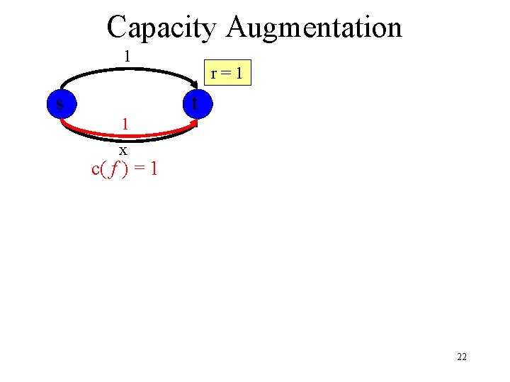
Capacity Augmentation 1 s 1 x r=1 t c( f ) = 1 22
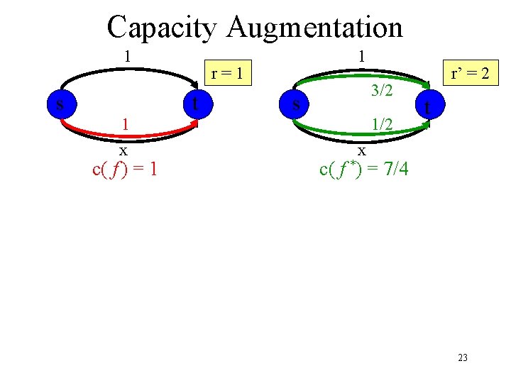
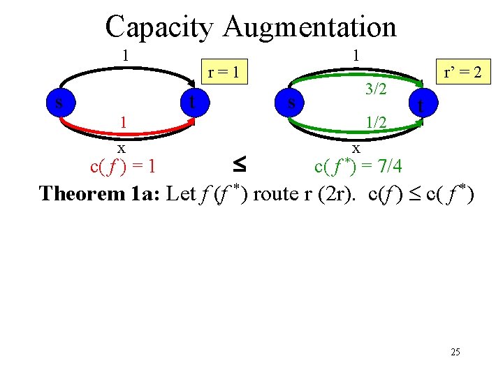
Capacity Augmentation 1 s 1 x c( f ) = 1 1 r=1 t 3/2 s 1/2 r’ = 2 t x c( f *) = 7/4 23
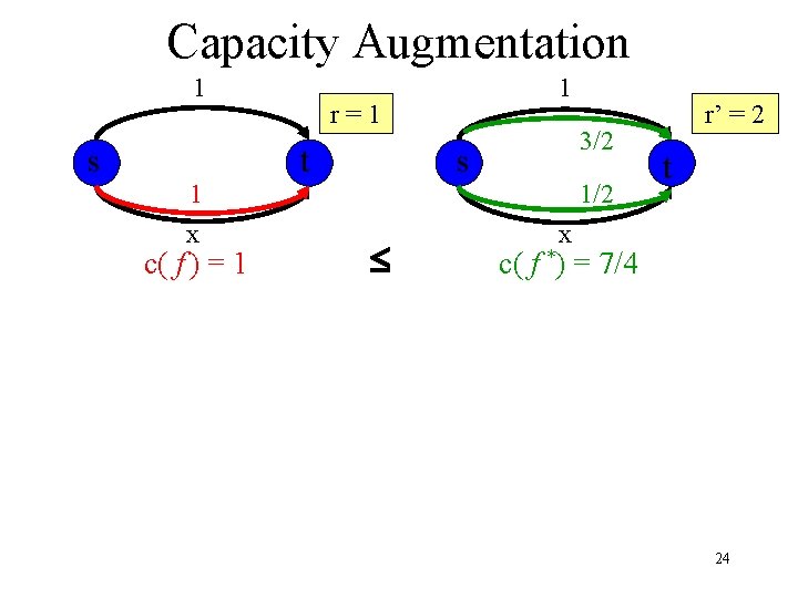
Capacity Augmentation 1 s 1 x c( f ) = 1 1 r=1 t 3/2 s 1/2 r’ = 2 t x c( f *) = 7/4 24
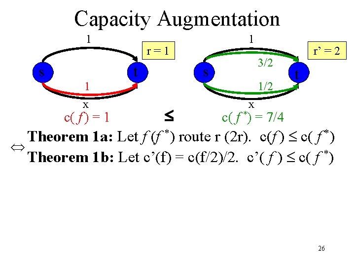
Capacity Augmentation 1 s 1 x 1 r=1 t 3/2 s 1/2 r’ = 2 t x c( f *) = 7/4 Theorem 1 a: Let f (f *) route r (2 r). c(f ) c( f *) c( f ) = 1 25
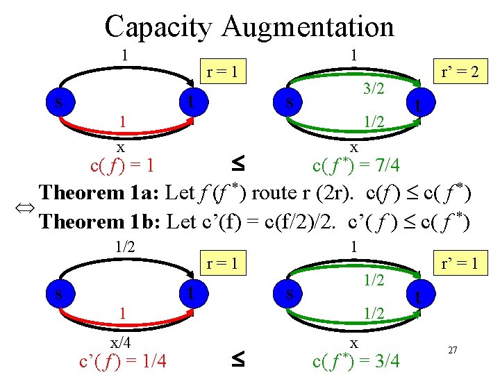
Capacity Augmentation 1 s 1 x 1 r=1 t 3/2 s 1/2 r’ = 2 t x c( f *) = 7/4 Theorem 1 a: Let f (f *) route r (2 r). c(f ) c( f *) Theorem 1 b: Let c’(f) = c(f/2)/2. c’( f ) c( f *) c( f ) = 1 26
Capacity Augmentation 1 s 1 x 1 r=1 t 3/2 s 1/2 r’ = 2 t x c( f *) = 7/4 Theorem 1 a: Let f (f *) route r (2 r). c(f ) c( f *) Theorem 1 b: Let c’(f) = c(f/2)/2. c’( f ) c( f *) c( f ) = 1 1/2 s 1 x/4 c’( f ) = 1/4 1 r=1 t 1/2 s 1/2 c( x f *) = 3/4 r’ = 1 t 27
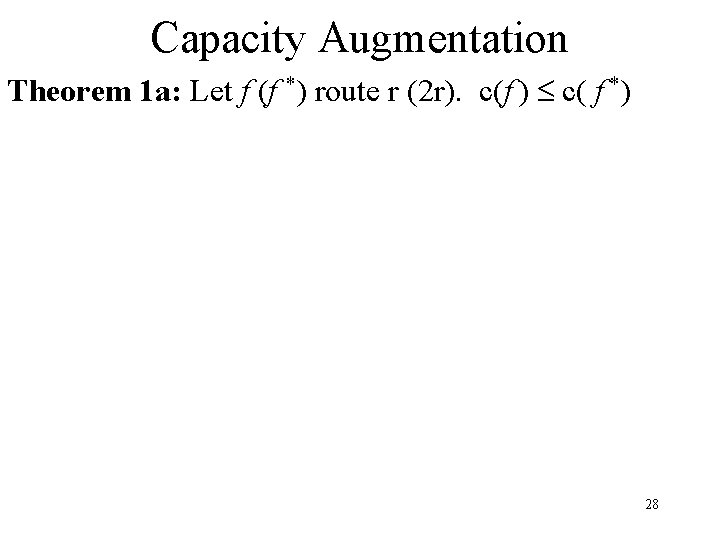
Capacity Augmentation Theorem 1 a: Let f (f *) route r (2 r). c(f ) c( f *) 28
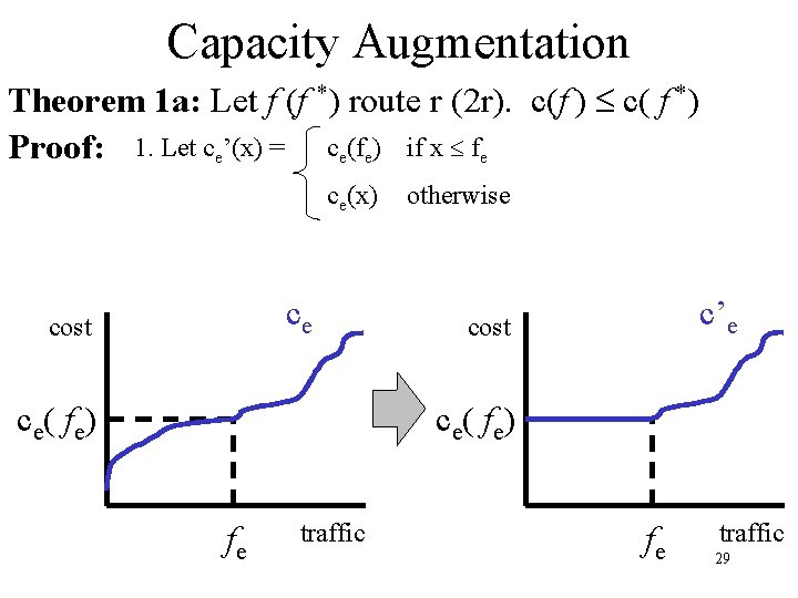
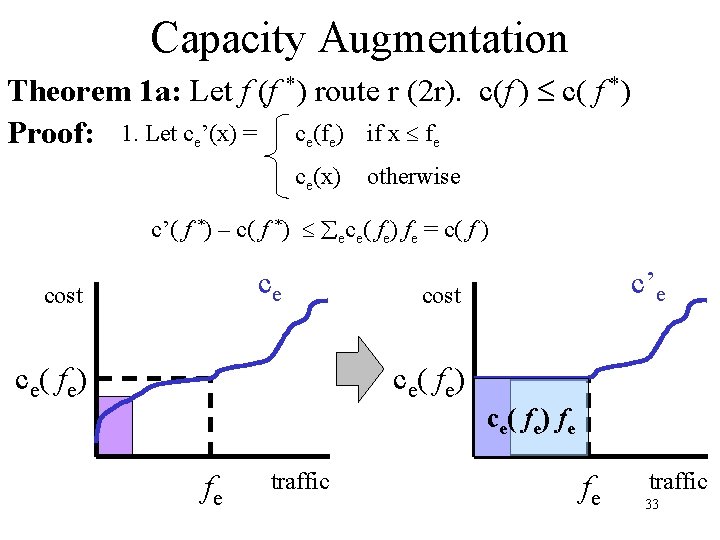
Capacity Augmentation Theorem 1 a: Let f (f *) route r (2 r). c(f ) c( f *) Proof: 1. Let ce’(x) = ce(fe) if x fe ce(x) ce cost c e( f e) otherwise c’e cost c e( f e) fe traffic 29
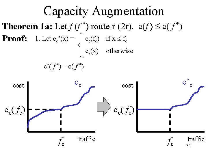
Capacity Augmentation Theorem 1 a: Let f (f *) route r (2 r). c(f ) c( f *) Proof: 1. Let ce’(x) = ce(fe) if x fe ce(x) otherwise c’( f *) – c( f *) ce cost c e( f e) c’e cost c e( f e) fe traffic 30
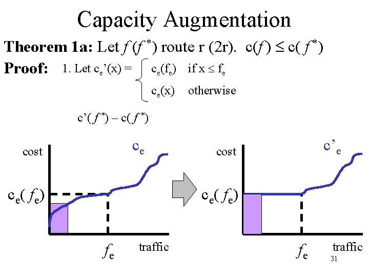
Capacity Augmentation Theorem 1 a: Let f (f *) route r (2 r). c(f ) c( f *) Proof: 1. Let ce’(x) = ce(fe) if x fe ce(x) otherwise c’( f *) – c( f *) ce cost c e( f e) c’e cost c e( f e) fe traffic 31
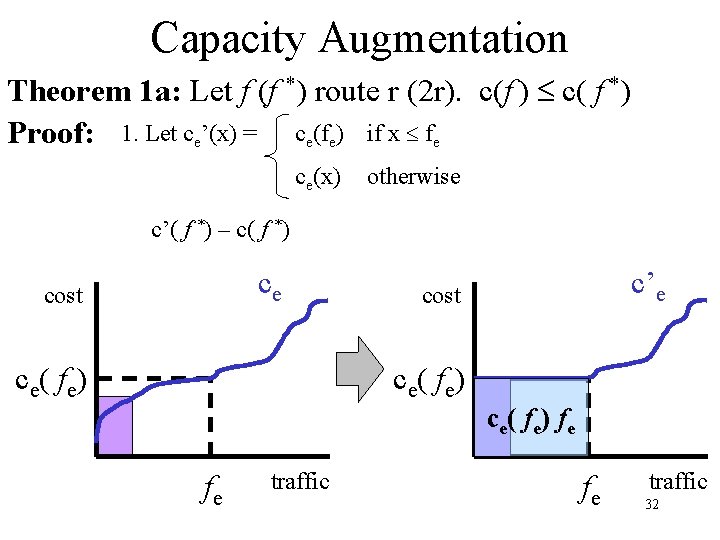
Capacity Augmentation Theorem 1 a: Let f (f *) route r (2 r). c(f ) c( f *) Proof: 1. Let ce’(x) = ce(fe) if x fe ce(x) otherwise c’( f *) – c( f *) ce cost c e( f e) c’e cost c e( f e) c e ( fe ) fe fe traffic 32
Capacity Augmentation Theorem 1 a: Let f (f *) route r (2 r). c(f ) c( f *) Proof: 1. Let ce’(x) = ce(fe) if x fe ce(x) otherwise c’( f *) – c( f *) ece( fe) fe = c( f ) ce cost c e( f e) c’e cost c e( f e) c e ( fe ) fe fe traffic 33
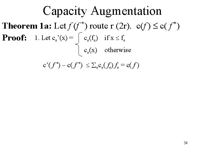
Capacity Augmentation Theorem 1 a: Let f (f *) route r (2 r). c(f ) c( f *) Proof: 1. Let ce’(x) = ce(fe) if x fe ce(x) otherwise c’( f *) – c( f *) ece( fe) fe = c( f ) 34
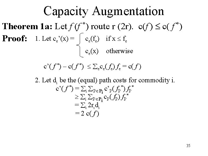
Capacity Augmentation Theorem 1 a: Let f (f *) route r (2 r). c(f ) c( f *) Proof: 1. Let ce’(x) = ce(fe) if x fe ce(x) otherwise c’( f *) – c( f *) ece( fe) fe = c( f ) 2. Let di be the (equal) path costs for commodity i. c’( f *) = i P Pi c’P( f. P*) f. P* i P Pi c. P( f. P) f. P* = i 2 ridi = 2 c( f ) 35
Capacity Augmentation Theorem 1 a: Let f (f *) route r (2 r). c(f ) c( f *) Proof: 1. Let ce’(x) = ce(fe) if x fe ce(x) otherwise c’( f *) – c( f *) ece( fe) fe = c( f ) 2. Let di be the (equal) path costs for commodity i. c’( f *) = i P Pi c’P( f. P*) f. P* i P Pi c. P( f. P) f. P* = i 2 ridi = 2 c( f ) 3. c( f*) c’( f *) - c( f ) 2 c( f ) - c( f ) = c( f ) (1) (2) 36
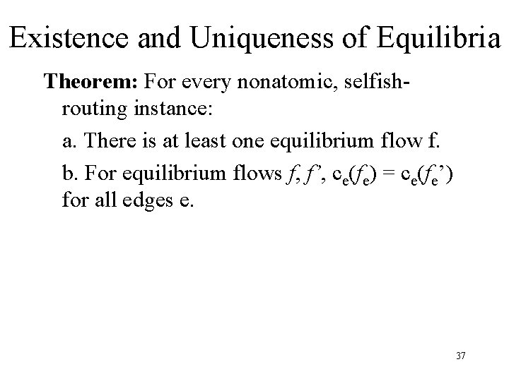
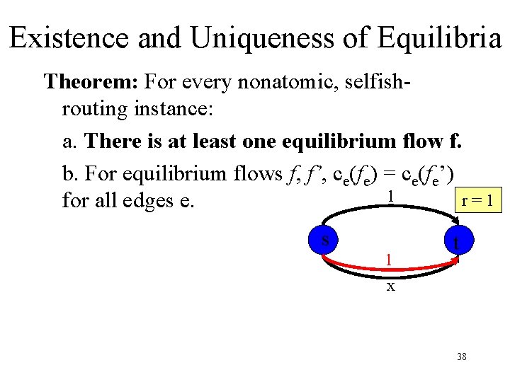
Existence and Uniqueness of Equilibria Theorem: For every nonatomic, selfishrouting instance: a. There is at least one equilibrium flow f. b. For equilibrium flows f, f’, ce(fe) = ce(fe’) for all edges e. 37
Existence and Uniqueness of Equilibria Theorem: For every nonatomic, selfishrouting instance: a. There is at least one equilibrium flow f. b. For equilibrium flows f, f’, ce(fe) = ce(fe’) 1 r=1 for all edges e. s 1 x t 38
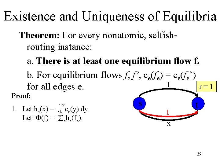
Existence and Uniqueness of Equilibria Theorem: For every nonatomic, selfishrouting instance: a. There is at least one equilibrium flow f. b. For equilibrium flows f, f’, ce(fe) = ce(fe’) 1 r=1 for all edges e. Proof: x 0 ce(y) 1. Let he(x) = dy. Let (f) = ehe(fe). s 1 x t 39
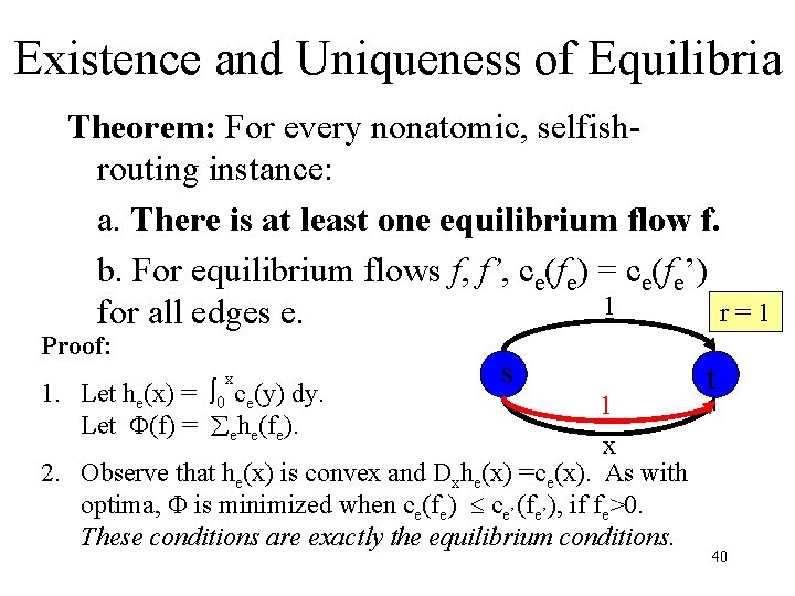
Existence and Uniqueness of Equilibria Theorem: For every nonatomic, selfishrouting instance: a. There is at least one equilibrium flow f. b. For equilibrium flows f, f’, ce(fe) = ce(fe’) 1 r=1 for all edges e. Proof: x 0 ce(y) 1. Let he(x) = dy. Let (f) = ehe(fe). s 1 x 2. Observe that he(x) is convex and Dxhe(x) =ce(x). As with optima, is minimized when ce(fe) ce’(fe’), if fe>0. These conditions are exactly the equilibrium conditions. t 40
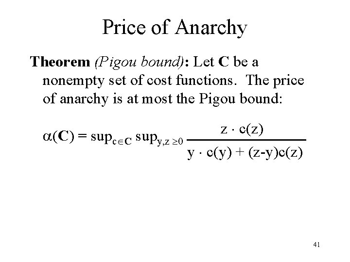
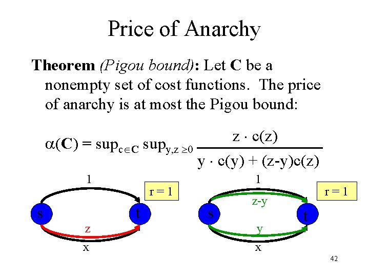
Price of Anarchy Theorem (Pigou bound): Let C be a nonempty set of cost functions. The price of anarchy is at most the Pigou bound: z c(z) (C) = supc C supy, z 0 y c(y) + (z-y)c(z) 41
Price of Anarchy Theorem (Pigou bound): Let C be a nonempty set of cost functions. The price of anarchy is at most the Pigou bound: z c(z) (C) = supc C supy, z 0 y c(y) + (z-y)c(z) 1 s z x 1 r=1 t s z-y y x r=1 t 42
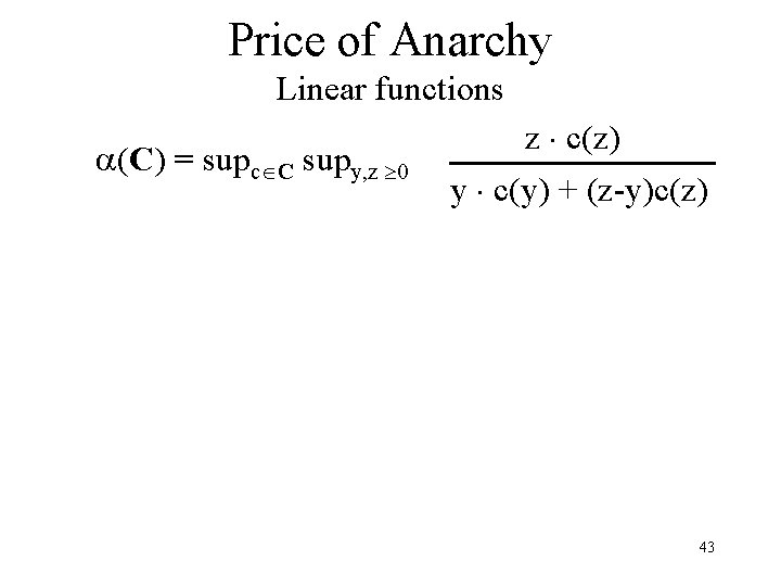
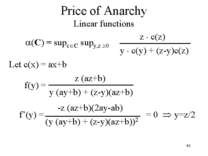
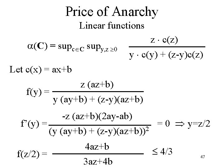
Price of Anarchy Linear functions (C) = supc C supy, z 0 z c(z) y c(y) + (z-y)c(z) 43
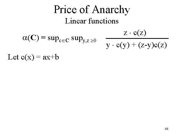
Price of Anarchy Linear functions (C) = supc C supy, z 0 z c(z) y c(y) + (z-y)c(z) Let c(x) = ax+b 44
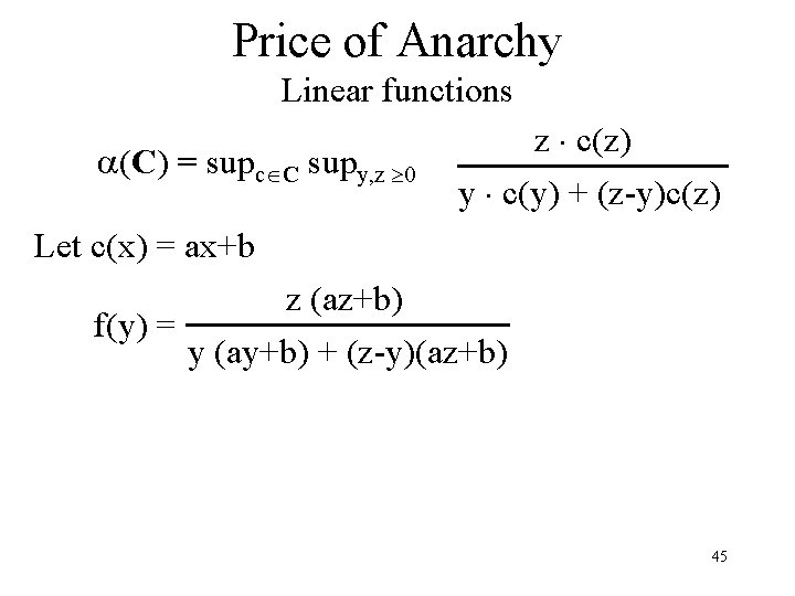
Price of Anarchy Linear functions (C) = supc C supy, z 0 z c(z) y c(y) + (z-y)c(z) Let c(x) = ax+b z (az+b) f(y) = y (ay+b) + (z-y)(az+b) 45
Price of Anarchy Linear functions (C) = supc C supy, z 0 z c(z) y c(y) + (z-y)c(z) Let c(x) = ax+b z (az+b) f(y) = y (ay+b) + (z-y)(az+b) -z (az+b)(2 ay-ab) f’(y) = = 0 y=z/2 (y (ay+b) + (z-y)(az+b))2 46
Price of Anarchy Linear functions (C) = supc C supy, z 0 z c(z) y c(y) + (z-y)c(z) Let c(x) = ax+b z (az+b) f(y) = y (ay+b) + (z-y)(az+b) -z (az+b)(2 ay-ab) f’(y) = = 0 y=z/2 (y (ay+b) + (z-y)(az+b))2 f(z/2) = 4 az+b 3 az+4 b 4/3 47
Other questions • Design good networks • Detect Braess’s paradox • Design mechanism to achieve social optimum • Confluent flows 48