Econ 427 lecture 18 slides Multivariate Modeling cntd

Econ 427 lecture 18 slides Multivariate Modeling (cntd) Byron Gangnes

Multivariate Forecasting • • Last time, we began discussing models where the evolution of one variable is related to developments in others This is suggested by much of our theory, and exploiting this can improve forecastsmultivariate regression modeling. Byron Gangnes

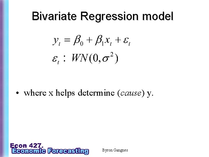
Bivariate Regression model • where x helps determine (cause) y. Byron Gangnes

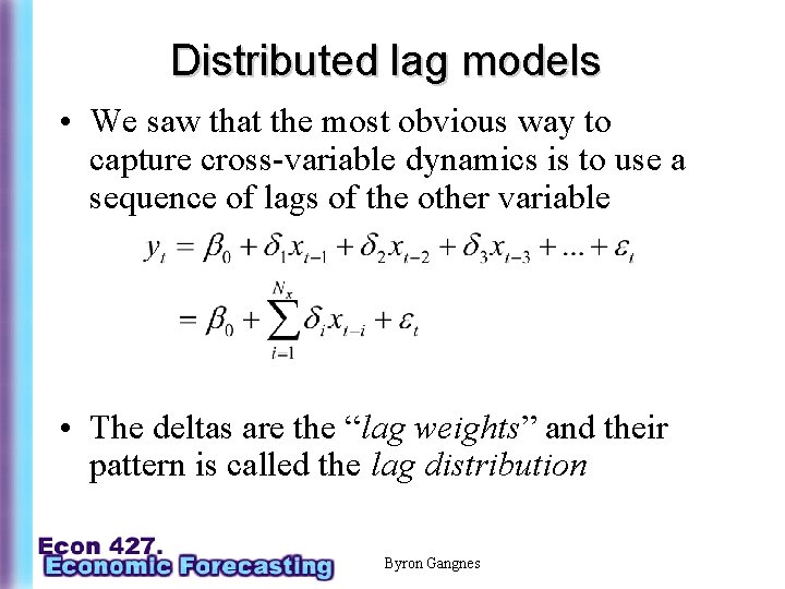
Distributed lag models • We saw that the most obvious way to capture cross-variable dynamics is to use a sequence of lags of the other variable • The deltas are the “lag weights” and their pattern is called the lag distribution Byron Gangnes

Estimation problems • Own-variable dynamics will usually also be important. We looked at different ways to handle that – – lag dependent variables. include ARMA disturbance Byron Gangnes

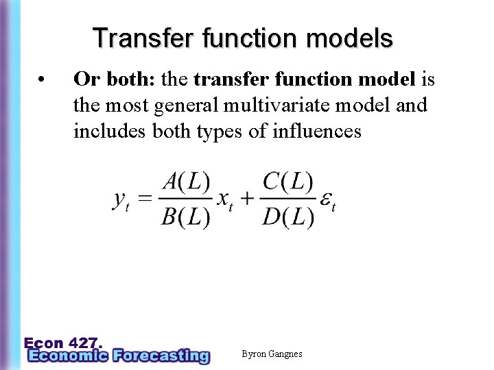
Transfer function models • Or both: the transfer function model is the most general multivariate model and includes both types of influences Byron Gangnes

Single or system equation models? • In some cases it may make sense to assume that right-hand side variables can be treated as exogenous for the purposes of modeling/forecasting a left-hand side variable – – E. g. an individual firms revenues may depend on GDP, but not visa versa. Formally what is needed for estimation (forecasting) is that the RHS var is weakly (strongly) exogenous with respect to the parameters we are trying to estimate. Byron Gangnes

Exogeneity concepts • A variable is weakly exogenous for parameters of interest if the marginal process for the variable contains no information useful for estimating those parameters – The marginal process is very roughly speaking the distribution of the variable itself without regard to particular values of variables it may be correlated with. – This means we can estimate the parameters without having to worry about the random process behind the weakly exogenous right-hand-side variable. • A variable is strongly exogenous if it is weakly exogenous AND it is not affected by lagged values of the endogenous variable. – In this case, we can forecast without having to worry about how our left-hand-side variable might affect future values of our righthand-side variable. Byron Gangnes

Single or system equation models? • Often, though, we want to allow for influences running potentially in both (all) directions – System modeling approaches Byron Gangnes

Vector Autoregressions (VAR) Byron Gangnes

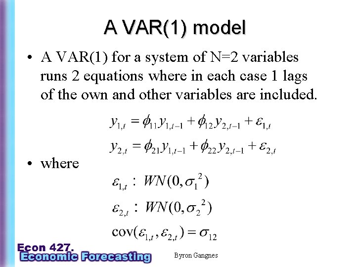
A VAR(1) model • A VAR(1) for a system of N=2 variables runs 2 equations where in each case 1 lags of the own and other variables are included. • where Byron Gangnes

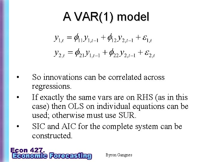
A VAR(1) model • • • So innovations can be correlated across regressions. If exactly the same vars are on RHS (as in this case) then OLS on individual equations can be used; otherwise must use SUR. SIC and AIC for the complete system can be constructed. Byron Gangnes

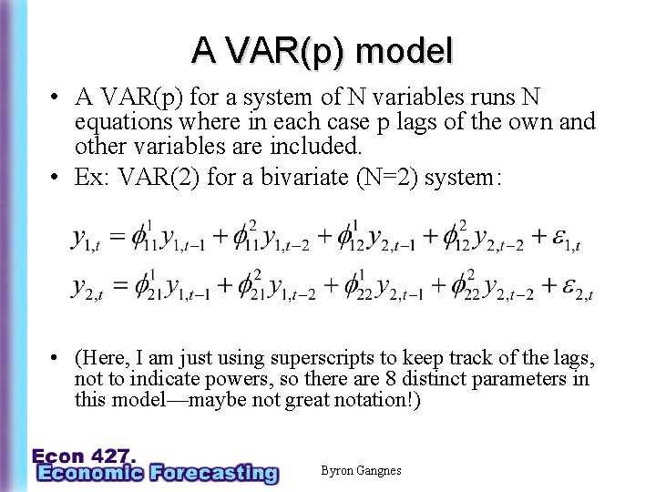
A VAR(p) model • A VAR(p) for a system of N variables runs N equations where in each case p lags of the own and other variables are included. • Ex: VAR(2) for a bivariate (N=2) system: • (Here, I am just using superscripts to keep track of the lags, not to indicate powers, so there are 8 distinct parameters in this model—maybe not great notation!) Byron Gangnes

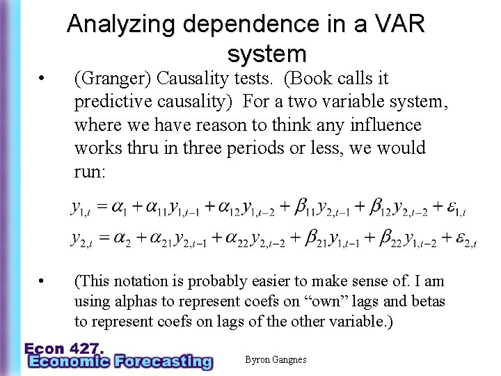
• • Analyzing dependence in a VAR system (Granger) Causality tests. (Book calls it predictive causality) For a two variable system, where we have reason to think any influence works thru in three periods or less, we would run: (This notation is probably easier to make sense of. I am using alphas to represent coefs on “own” lags and betas to represent coefs on lags of the other variable. ) Byron Gangnes

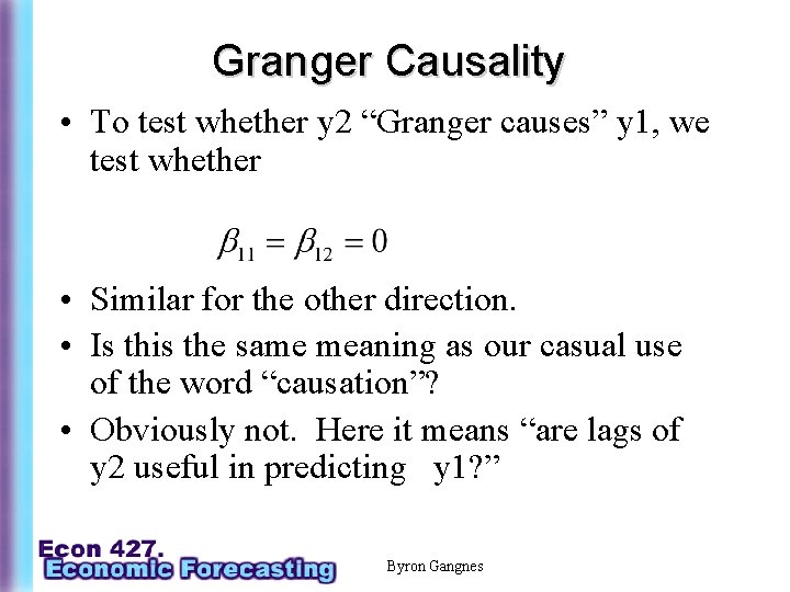
Granger Causality • To test whether y 2 “Granger causes” y 1, we test whether • Similar for the other direction. • Is this the same meaning as our casual use of the word “causation”? • Obviously not. Here it means “are lags of y 2 useful in predicting y 1? ” Byron Gangnes

Impulse-response functions • • • We use impulse-response functions to see how a shock to the variables affect each other. We want to know how an innovation in one of the variables will affect itself over time and the other variable(s). Next time… Byron Gangnes