Econ 427 lecture 21 slides Nonstationary data series
- Slides: 18

Econ 427 lecture 21 slides Non-stationary data series Byron Gangnes

Announcements • I will be away tonight thru Sunday • Thursday I am giving you the class period to work on your projects • You need to “check in” that day, but I will not force you to come to campus. So either: – Show up in class and sign in with my TA, Xiaodong Sun, or – Send him an email to let him know you will not be there: sun 9@hawaii. edu Byron Gangnes

Announcements • I am rearranging material – We will cover non-stationary time series this week and next (Ch. 13) – Then we will go back and cover Ch. 12 on evaluating and combining forecasts Byron Gangnes

Covariance Stationary series • • We know the statistical basis for our estimation and forecasting depends on series being covariance stationary. Actually we have modeled some non-stationary behavior. What kind? Models with deterministic trends. e. g. ARMA(1, 1) with constant and trend: Essentially we are using OLS to “detrend” the series so that the remaining stochastic process is stationary. Byron Gangnes

Non-stationary series • • An alternative that describes well some economic, financial and business data is to allow a random (stochastic) trend. Turns out that data having such trends may need to be handled in a different way. Byron Gangnes

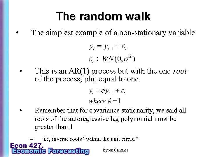
The random walk • The simplest example of a non-stationary variable • This is an AR(1) process but with the one root of the process, phi, equal to one. • Remember that for covariance stationarity, we said all roots of the autoregressive lag polynomial must be greater than 1 – i. e, inverse roots “within the unit circle. ” Byron Gangnes

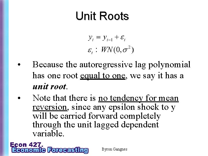
Unit Roots • • Because the autoregressive lag polynomial has one root equal to one, we say it has a unit root. Note that there is no tendency for mean reversion, since any epsilon shock to y will be carried forward completely through the unit lagged dependent variable. Byron Gangnes

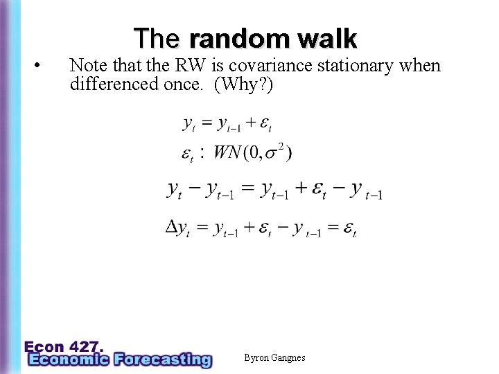
• The random walk Note that the RW is covariance stationary when differenced once. (Why? ) Byron Gangnes

Integrated series • • • Terminology: we say that yt is integrated of order 1, I(1) “eye-one”, because it has to be differenced once to get a stationary time series. In general a series can be I(d), if it must be differenced d times to get a stationary series. Some I(2) series occur (the price level may be one), but most common are I(1) or I(0) (series that are already cov. stationary without any differencing. ) Byron Gangnes

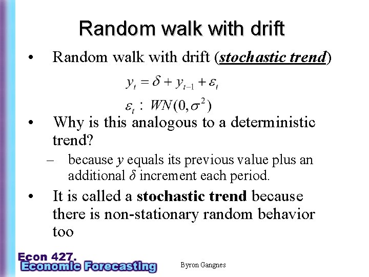
Random walk with drift • Random walk with drift (stochastic trend) • Why is this analogous to a deterministic trend? – because y equals its previous value plus an additional δ increment each period. • It is called a stochastic trend because there is non-stationary random behavior too Byron Gangnes

Examples • Look at the examples of simulated random walk and random walk with drift series in EViews (also see in the book pp. 290 -291) – – Can you see why it might be difficult in practice to distinguish between ARMA models with deterministric trend and stochastic trends (unit roots)? We have seen that ARMA models (AR in particular) can generate trending cyclical patterns with a lot of persistence, that look similar to random walks. Byron Gangnes

Problems with Unit Roots • Because they are not covariance stationary (we’ll come back to this next week) unit roots require some special treatment. – – – Statistically, the existence of unit roots can be problematic because OLS estimates of the AR(1) coef. phi are biased downward. In multivariate frameworks, one can get spurious regression results So we may want to test whether a unit root exists. Byron Gangnes

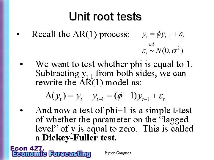
Unit root tests • Recall the AR(1) process: • We want to test whether phi is equal to 1. Subtracting yt-1 from both sides, we can rewrite the AR(1) model as: • And now a test of phi=1 is a simple t-test of whether the parameter on the “lagged level” of y is equal to zero. This is called a Dickey-Fuller test. Byron Gangnes

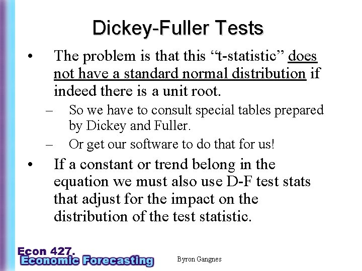
Dickey-Fuller Tests • The problem is that this “t-statistic” does not have a standard normal distribution if indeed there is a unit root. – – • So we have to consult special tables prepared by Dickey and Fuller. Or get our software to do that for us! If a constant or trend belong in the equation we must also use D-F test stats that adjust for the impact on the distribution of the test statistic. Byron Gangnes

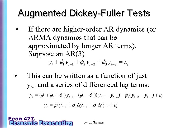
Augmented Dickey-Fuller Tests • If there are higher-order AR dynamics (or ARMA dynamics that can be approximated by longer AR terms). Suppose an AR(3) • This can be written as a function of just yt-1 and a series of differenced lag terms: Byron Gangnes

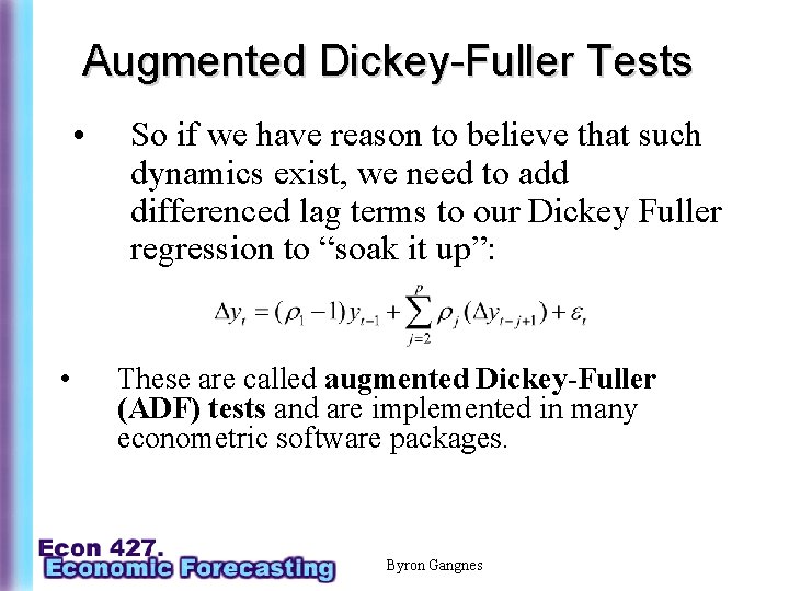
Augmented Dickey-Fuller Tests • • So if we have reason to believe that such dynamics exist, we need to add differenced lag terms to our Dickey Fuller regression to “soak it up”: These are called augmented Dickey-Fuller (ADF) tests and are implemented in many econometric software packages. Byron Gangnes

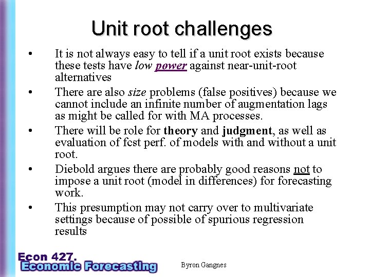
Unit root challenges • • • It is not always easy to tell if a unit root exists because these tests have low power against near-unit-root alternatives There also size problems (false positives) because we cannot include an infinite number of augmentation lags as might be called for with MA processes. There will be role for theory and judgment, as well as evaluation of fcst perf. of models with and without a unit root. Diebold argues there are probably good reasons not to impose a unit root (model in differences) forecasting work. This presumption may not carry over to multivariate settings because of possible of spurious regression results Byron Gangnes

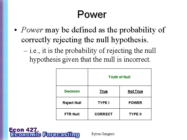
Power • Power may be defined as the probability of correctly rejecting the null hypothesis. – i. e. , it is the probability of rejecting the null hypothesis given that the null is incorrect. Truth of Null Decision True Not True Reject Null TYPE I POWER FTR Null CORRECT TYPE II Byron Gangnes