Ag Econ 635 Topics in Consumer Demand Analysis

Ag Econ 635 Topics in Consumer Demand Analysis Dr. Oral Capps, Jr. Texas A&M University Spring 2008

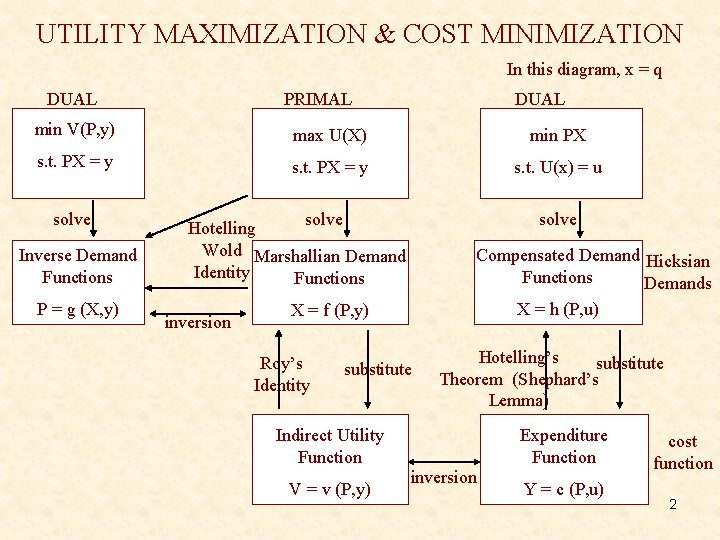
UTILITY MAXIMIZATION & COST MINIMIZATION In this diagram, x = q DUAL PRIMAL DUAL min V(P, y) max U(X) min PX s. t. PX = y s. t. U(x) = u solve Inverse Demand Functions P = g (X, y) solve Hotelling Wold Marshallian Demand Identity Functions inversion solve Compensated Demand Hicksian Functions Demands X = h (P, u) X = f (P, y) Roy’s Identity substitute Hotelling’s substitute Theorem (Shephard’s Lemma) Indirect Utility Function V = v (P, y) Expenditure Function inversion Y = c (P, u) cost function 2

Stigler – Early history of empirical studies of consumer behavior Ø Modern Era of Budgentary Studies Ø Key development Ø Popularization of statistical snalyses of collections of social data Ø Adolphe Quetelet – Chief Exponent of the application of statistical techniques to social data – 1869 Ø Engel – First and most famous of all statistical analyses of budgets – 1857 Ø Engel’s Law Ø The budget share for food declines with increases in disposable income Ø True today? 3

Illustration of Engel’s Law for Total Food Expenditures 4

--Engel – development of adult equivalence scale - basic unit of measurement “quet” in honor of Quetelet --Schwabe’s Law 1868 - the budget share for housing rises with decreases in disposable income --Wright’s Law 1875 -the higher the income, the greater the saving --By the 1870 s, budget studies an established area of work. 5

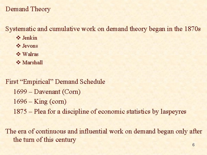
Demand Theory Systematic and cumulative work on demand theory began in the 1870 s v Jenkin v Jevons v Walras v Marshall First “Empirical” Demand Schedule 1699 – Davenant (Corn) 1696 – King (corn) 1875 – Plea for a discipline of economic statistics by laspeyres The era of continuous and influential work on demand began only after the turn of this century 6

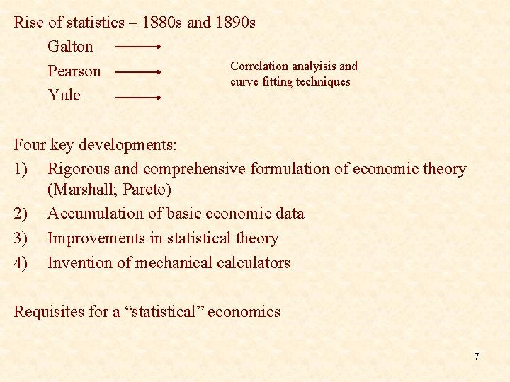
Rise of statistics – 1880 s and 1890 s Galton Correlation analyisis and Pearson curve fitting techniques Yule Four key developments: 1) Rigorous and comprehensive formulation of economic theory (Marshall; Pareto) 2) Accumulation of basic economic data 3) Improvements in statistical theory 4) Invention of mechanical calculators Requisites for a “statistical” economics 7

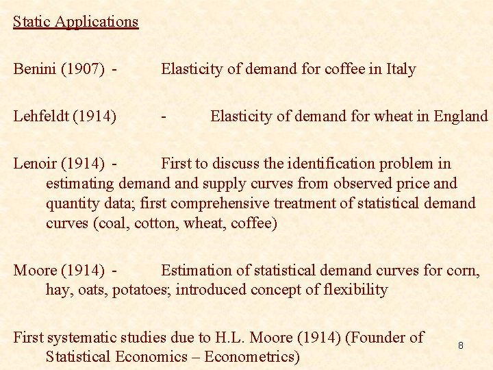
Static Applications Benini (1907) - Elasticity of demand for coffee in Italy Lehfeldt (1914) - Elasticity of demand for wheat in England Lenoir (1914) First to discuss the identification problem in estimating demand supply curves from observed price and quantity data; first comprehensive treatment of statistical demand curves (coal, cotton, wheat, coffee) Moore (1914) Estimation of statistical demand curves for corn, hay, oats, potatoes; introduced concept of flexibility First systematic studies due to H. L. Moore (1914) (Founder of Statistical Economics – Econometrics) 8

Allen & Bowley (1935) Consumer demand studied as a function of income and socio-demographic characteristics; analysis based on household budget data Family Expenditure Schultz (1938)income Study of demand as a function of prices and Theory and Measurement of Demand Wold and Jureen (1938– 1940) Combine the analysis of family budget data and time-series data to obtain a unified picture of the demand structure in Sweden in 1920 -1938. “In demand analysis, empirical and theoretical inference are interwoven, economic theory being used for guiding and supporing the statistical methods and checking the empirical findings” 9

Articles by Elmer Working and by Haavelmo spelled out the reasons why the usual least squares analysis may not result in a true demand curve of economic theory. Since these theoretical articles, various statistical methods have been developed to try to estimate true demand curves. Stone (1954, 1958) – Demand analysis in Great Britain which covered somewhat the same ground as that covered by the Schultz analysis in the U. S. ; Demand Systems (Linear Expenditure System) Earliest example of the specification and estimation of complete demand systems (Leser (1941)). 1940 s, 1950 s Foote – Simultaneous demand supply equations Nerlove – Distributed Lag Models Fox – Recursive System of Equations 10

1960 s, 1970 s Complete Demand Systems Model. Pioneering efforts by Frisch (1959), Houthakker (1960), Stone, Strotz, Brandow, George and King, Bieri and De. Janvry, Barten, Theil, Powell, Goldberger Demand analysis is a field where statistical data are relatively plentiful and reliable. Empirical demand analysis in the 1970 s and 1980 s more problem oriented than in the past. Flurry of empirical analysis on demand systems past 20 -25 years. Advancements in computational technology. Current Pursuits Dynamic Applications Extensions of Neoclassical Theory 11

Interdependent Nature of Demand A “complete” matrix of elasticities use of restrictions on elasticities v. Homogeneity condition v. Symmetry (Slutsky) Condition v. Engel Aggregation v. Cournot Aggregation v. Additivity (Frisch Equations) v. Ordinal Separability Conditions Brandow George and King Huang Demand Systems Literature 12

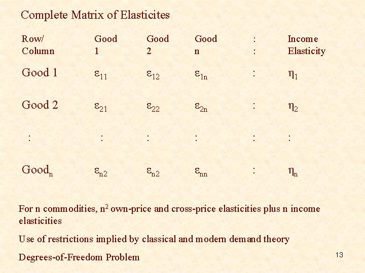
Complete Matrix of Elasticites Row/ Column Good 1 Good 2 Good n : : Income Elasticity Good 1 ε 12 ε 1 n : η 1 Good 2 ε 21 ε 22 ε 2 n : η 2 : : εn 2 εnn : ηn : Goodn : εn 2 For n commodities, n 2 own-price and cross-price elasticities plus n income elasticities Use of restrictions implied by classical and modern demand theory Degrees-of-Freedom Problem 13

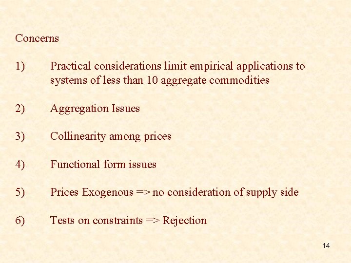
Concerns 1) Practical considerations limit empirical applications to systems of less than 10 aggregate commodities 2) Aggregation Issues 3) Collinearity among prices 4) Functional form issues 5) Prices Exogenous => no consideration of supply side 6) Tests on constraints => Rejection 14

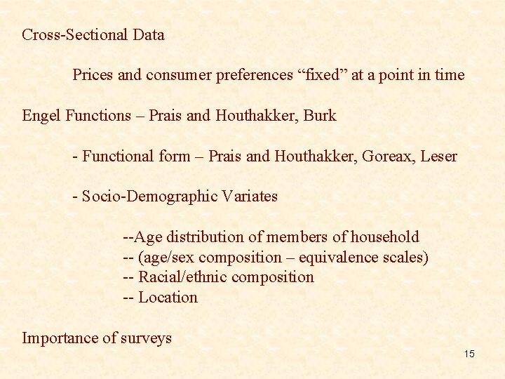
Cross-Sectional Data Prices and consumer preferences “fixed” at a point in time Engel Functions – Prais and Houthakker, Burk - Functional form – Prais and Houthakker, Goreax, Leser - Socio-Demographic Variates --Age distribution of members of household -- (age/sex composition – equivalence scales) -- Racial/ethnic composition -- Location Importance of surveys 15

Measures of Consumption --Expenditures --Quantities Quality, Quantity, and Expenditure Elasticities Measures of Income --Total Expenditures --Gross Income --DPI --Imputations from home-grown food, transfer payments, income subsidies --MPCs out of different types of income --Food Stamp --School Lunch Programs --School Breakfast 16

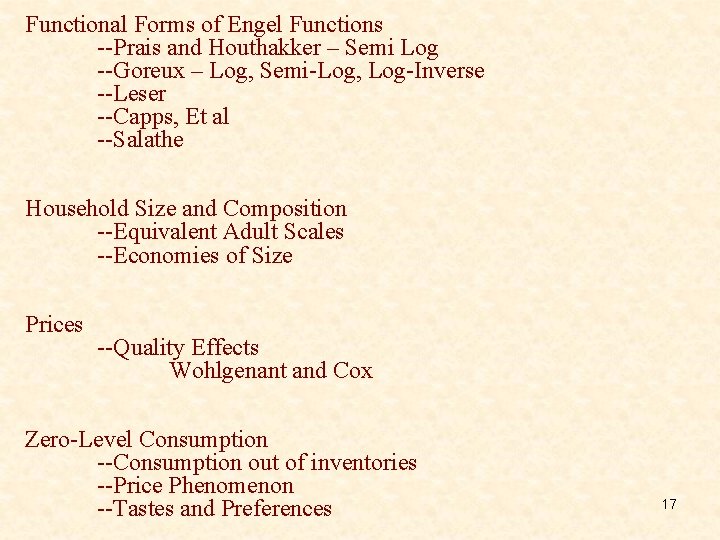
Functional Forms of Engel Functions --Prais and Houthakker – Semi Log --Goreux – Log, Semi-Log, Log-Inverse --Leser --Capps, Et al --Salathe Household Size and Composition --Equivalent Adult Scales --Economies of Size Prices --Quality Effects Wohlgenant and Cox Zero-Level Consumption --Consumption out of inventories --Price Phenomenon --Tastes and Preferences 17

Given that a well-behaved utility function represents a given preference ofdering, a reasonable question to ask: “Is this representation unique? ” No – a family of transformations can do equally well to represent the same preference ordering. Ordinalism Versus Cardinalism A measure is said to be cardinal when it is subject to linear (increasing) transformations only. It is ordinal when all monotonic (increasing) transformations are allowed. Menger, Gossen, Walras – Cardinal Nature of Utility Functions Fisher, Pareto, Hicks – Ordinal Nature of Utility Functions Utility function is always defined as ordinal – much less restrictive and not realistic to suppose that satisfaction is measureable in a cardinal way. Defining the axioms necessary for establishing the existence of a well-behaved utility function has laid the foundations for the ordinal 18 approach.

Exercise 1. 7 -- Phlips Suppose a utility function in terms of specified as and is Let there also be the following utility functions: (A) Which functions are transformations of (1)? is not a transformation of U (B) Cardinal measures 19

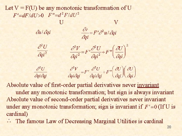
Let V = F(U) be any monotonic transformation of U U V Absolute value of first-order partial derivatives never invariant under any monotonic transformation; but sign is always invariant Absolute value of second-order partial derivatives never invariant under any monotonic transformation; sign is invariant if (If U is cardinal) The famous Law of Decreasing Marginal Utilities is cardinal 20

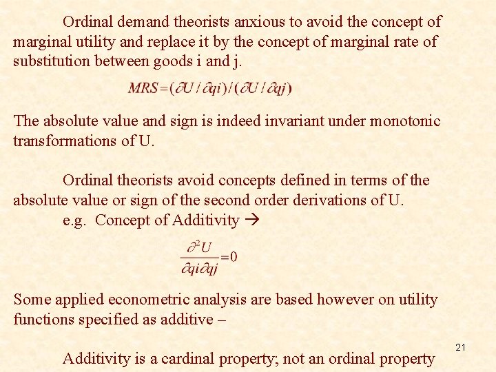
Ordinal demand theorists anxious to avoid the concept of marginal utility and replace it by the concept of marginal rate of substitution between goods i and j. The absolute value and sign is indeed invariant under monotonic transformations of U. Ordinal theorists avoid concepts defined in terms of the absolute value or sign of the second order derivations of U. e. g. Concept of Additivity Some applied econometric analysis are based however on utility functions specified as additive – Additivity is a cardinal property; not an ordinal property 21

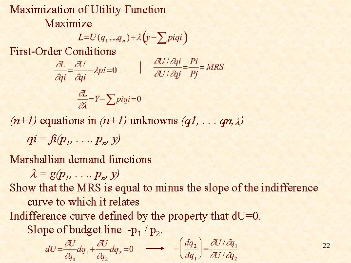
Maximization of Utility Function Maximize First-Order Conditions (n+1) equations in (n+1) unknowns (q 1, . . . qn, ) qi = fi(p 1, . . . , pn, y) Marshallian demand functions = g(p 1, . . . , pn, y) Show that the MRS is equal to minus the slope of the indifference curve to which it relates Indifference curve defined by the property that d. U=0. Slope of budget line -p 1 / p 2. 22

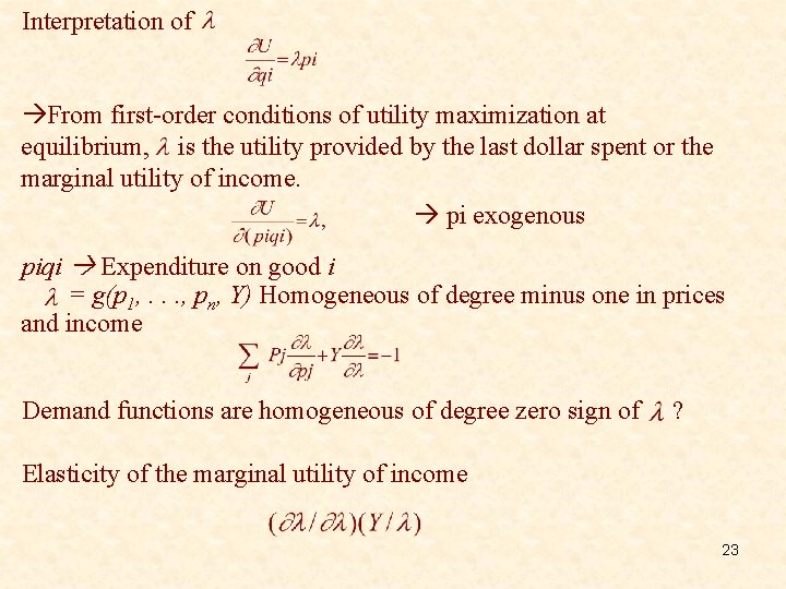
Interpretation of From first-order conditions of utility maximization at equilibrium, is the utility provided by the last dollar spent or the marginal utility of income. pi exogenous piqi Expenditure on good i = g(p 1, . . . , pn, Y) Homogeneous of degree minus one in prices and income Demand functions are homogeneous of degree zero sign of ? Elasticity of the marginal utility of income 23

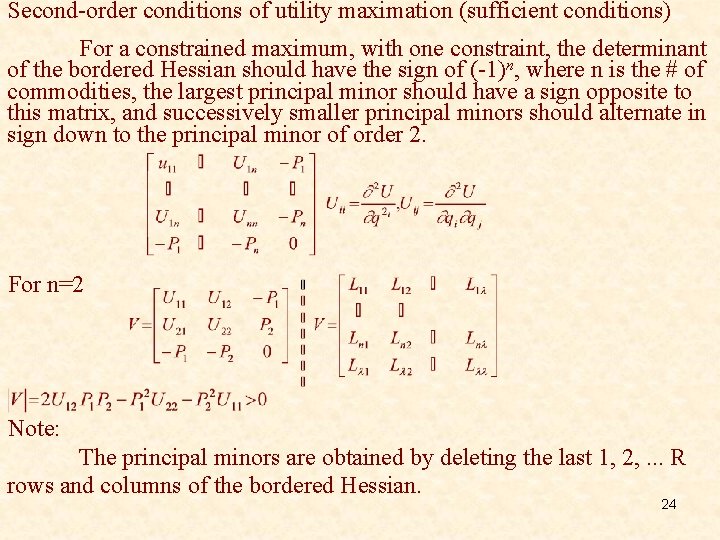
Second-order conditions of utility maximation (sufficient conditions) For a constrained maximum, with one constraint, the determinant of the bordered Hessian should have the sign of (-1)n, where n is the # of commodities, the largest principal minor should have a sign opposite to this matrix, and successively smaller principal minors should alternate in sign down to the principal minor of order 2. For n=2 Note: The principal minors are obtained by deleting the last 1, 2, . . . R rows and columns of the bordered Hessian. 24

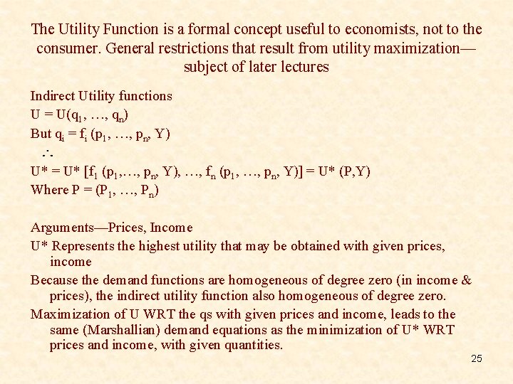
The Utility Function is a formal concept useful to economists, not to the consumer. General restrictions that result from utility maximization— subject of later lectures Indirect Utility functions U = U(q 1, …, qn) But qi = fi (p 1, …, pn, Y) U* = U* [f 1 (p 1, …, pn, Y), …, fn (p 1, …, pn, Y)] = U* (P, Y) Where P = (P 1, …, Pn) Arguments—Prices, Income U* Represents the highest utility that may be obtained with given prices, income Because the demand functions are homogeneous of degree zero (in income & prices), the indirect utility function also homogeneous of degree zero. Maximization of U WRT the qs with given prices and income, leads to the same (Marshallian) demand equations as the minimization of U* WRT prices and income, with given quantities. 25

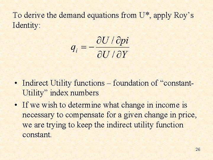
To derive the demand equations from U*, apply Roy’s Identity: • Indirect Utility functions – foundation of “constant. Utility” index numbers • If we wish to determine what change in income is necessary to compensate for a given change in price, we are trying to keep the indirect utility function constant. 26

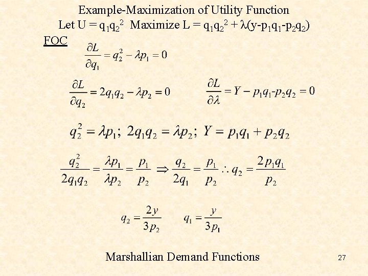
Example-Maximization of Utility Function Let U = q 1 q 22 Maximize L = q 1 q 22 + λ(y-p 1 q 1 -p 2 q 2) FOC Marshallian Demand Functions 27

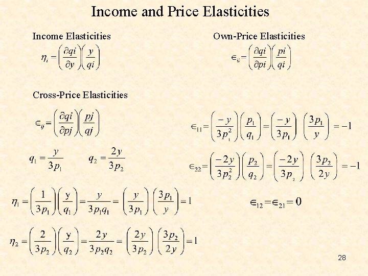
Income and Price Elasticities Income Elasticities Own-Price Elasticities Cross-Price Elasticities 28

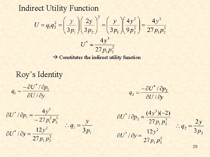
Indirect Utility Function Constitutes the indirect utility function Roy’s Identity 29

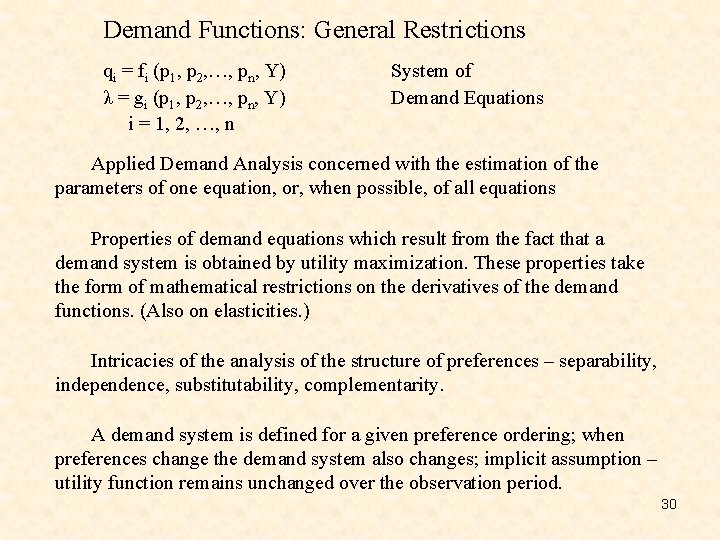
Demand Functions: General Restrictions qi = fi (p 1, p 2, …, pn, Y) λ = gi (p 1, p 2, …, pn, Y) i = 1, 2, …, n System of Demand Equations Applied Demand Analysis concerned with the estimation of the parameters of one equation, or, when possible, of all equations Properties of demand equations which result from the fact that a demand system is obtained by utility maximization. These properties take the form of mathematical restrictions on the derivatives of the demand functions. (Also on elasticities. ) Intricacies of the analysis of the structure of preferences – separability, independence, substitutability, complementarity. A demand system is defined for a given preference ordering; when preferences change the demand system also changes; implicit assumption – utility function remains unchanged over the observation period. 30

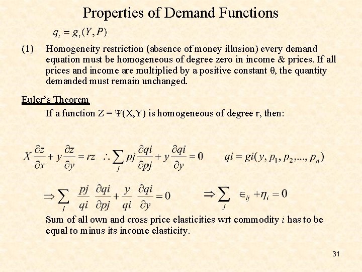
Properties of Demand Functions (1) Homogeneity restriction (absence of money illusion) every demand equation must be homogeneous of degree zero in income & prices. If all prices and income are multiplied by a positive constant θ, the quantity demanded must remain unchanged. Euler’s Theorem If a function Z = (X, Y) is homogeneous of degree r, then: Sum of all own and cross price elasticities wrt commodity i has to be equal to minus its income elasticity. 31

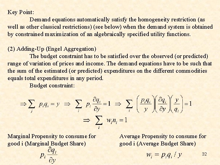
Key Point: Demand equations automatically satisfy the homogeneity restriction (as well as other classical restrictions) (see below) when the demand system is obtained by constrained maximization of an algebraically specified utility functions. (2) Adding-Up (Engel Aggregation) The budget constraint has to be satisfied over the observed (or predicted) range of variation of prices and income. The demand equations have to be such that the sum of the estimated (or predicted) expenditures on the different commodities equals total expenditures in any period. Budget constraint: Marginal Propensity to consume for good i (Marginal Budget Share) Average Propensity to consume for good i (Average Budget Share) 32

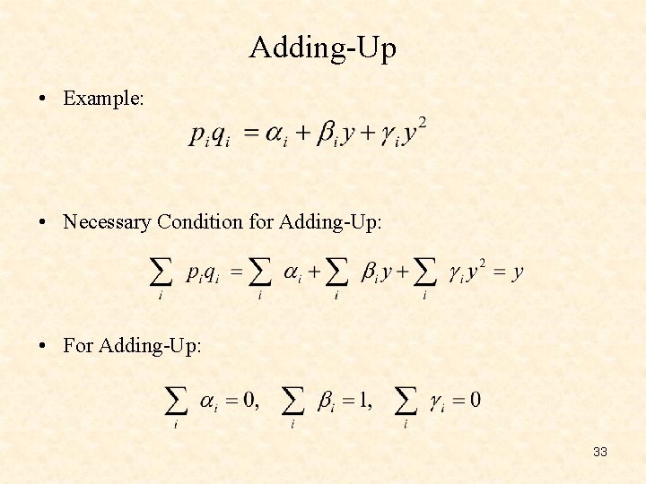
Adding-Up • Example: • Necessary Condition for Adding-Up: • For Adding-Up: 33

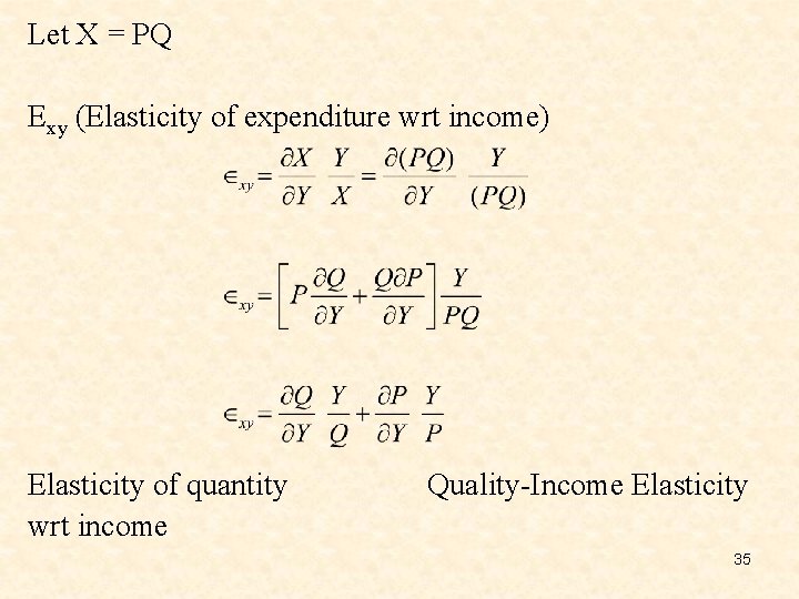
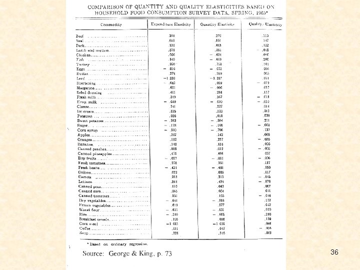
Distinguish between the response of quantity to income changes & that of expenditure to income changes (1) Quantity-income elasticities (2) Expenditure-income elasticities (3) Quality-income elasticities (% change in average price paid/unit due to a 1% change in income) George & King P. 72. A Measure of the quality consciousness of consumers Assumption: Quality of a product and price are positively correlated. 34

Let X = PQ Exy (Elasticity of expenditure wrt income) Elasticity of quantity wrt income Quality-Income Elasticity 35

36

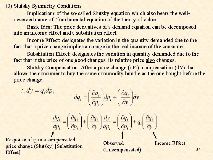
(3) Slutsky Symmetry Conditions Implications of the so-called Slutsky equation which also bears the welldeserved name of “fundamental equation of theory of value. ” Basic Idea: The price derivatives of a demand equation can be decomposed into an income effect and a substitution effect. Income Effect: designates the variation in the quantity demanded due to the fact that a price change implies a change in the real income of the consumer. Substitution Effect: designates the variation in quantity demanded due to the fact that if the price of one good changes, its relative price also changes. Slutsky Compensation: After a price change (d. Pi), compensation (d. Y) that allows the consumer to buy the same commodity bundle as the one bought before the price change. Response of qi to a compensated price change (Slutsky) [Substitution Effect] Observed (Uncompensated) Income Effect 37

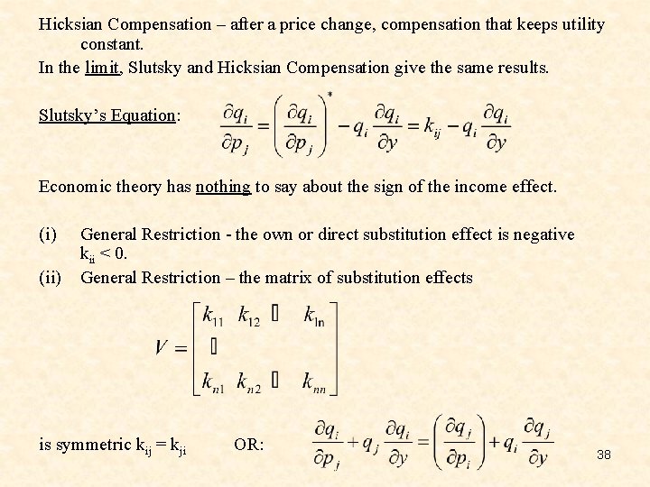
Hicksian Compensation – after a price change, compensation that keeps utility constant. In the limit, Slutsky and Hicksian Compensation give the same results. Slutsky’s Equation: Economic theory has nothing to say about the sign of the income effect. (i) (ii) General Restriction - the own or direct substitution effect is negative kii < 0. General Restriction – the matrix of substitution effects is symmetric kij = kji OR: 38

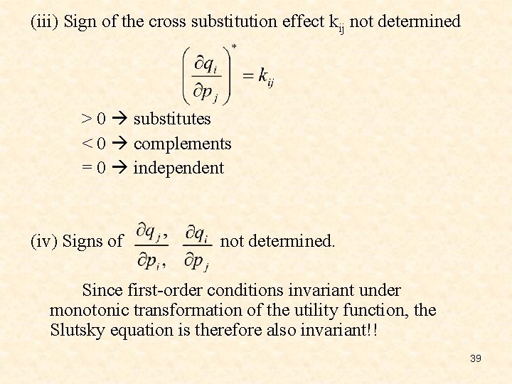
(iii) Sign of the cross substitution effect kij not determined > 0 substitutes < 0 complements = 0 independent (iv) Signs of not determined. Since first-order conditions invariant under monotonic transformation of the utility function, the Slutsky equation is therefore also invariant!! 39

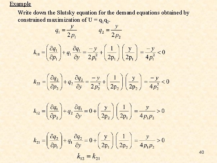
Example Write down the Slutsky equation for the demand equations obtained by constrained maximization of U = q 1 q 2. 40

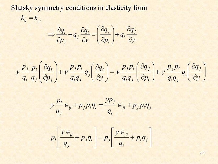
Slutsky symmetry conditions in elasticity form 41

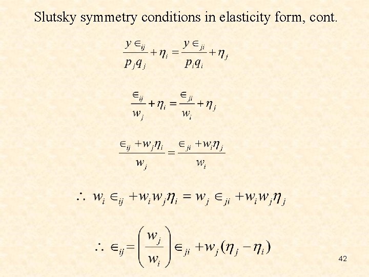
Slutsky symmetry conditions in elasticity form, cont. 42

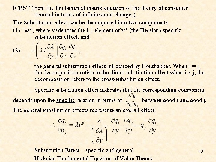
ICBST (from the fundamental matrix equation of theory of consumer demand in terms of infinitesimal changes) The Substitution effect can be decomposed into two components (1) λvij, where vij denotes the i, j element of v-1 (the Hessian) specific substitution effect, and (2) the general substitution effect introduced by Houthakker. When i = j, the decomposition refers to the direct substitution effect when i j, the decomposition refers to the cross-substitution effect. Specific substitution effect indicates that the corresponding component depends upon the specific relation in terms of between good i and good j. The general substitution effects represents an overall effect. Substitution Effect – specific and general Hicksian Fundamental Equation of Value Theory 43

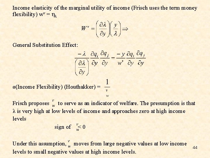
Income elasticity of the marginal utility of income (Frisch uses the term money flexibility) wv = General Substitution Effect: ø(Income Flexibility) (Houthakker) = Frisch proposes to serve as an indicator of welfare. The presumption is that λ is very high at low levels of income and approaches zero at high income levels sign of < 0 Under this assumption, moves from large negative values at low income levels to small negative values at high income levels. 44

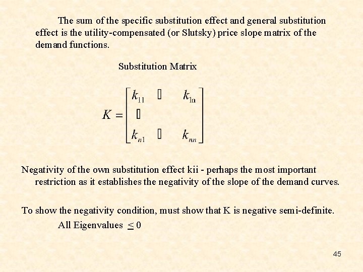
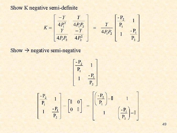
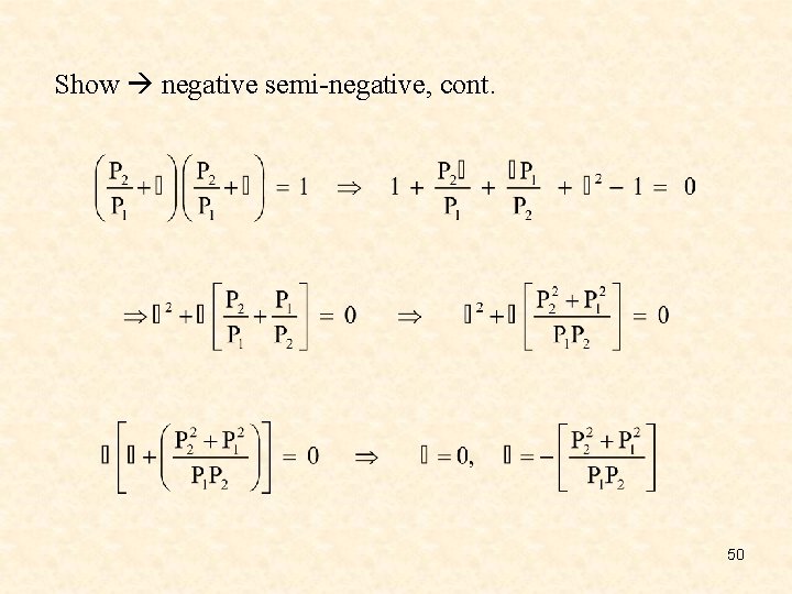
The sum of the specific substitution effect and general substitution effect is the utility-compensated (or Slutsky) price slope matrix of the demand functions. Substitution Matrix Negativity of the own substitution effect kii - perhaps the most important restriction as it establishes the negativity of the slope of the demand curves. To show the negativity condition, must show that K is negative semi-definite. All Eigenvalues < 0 45

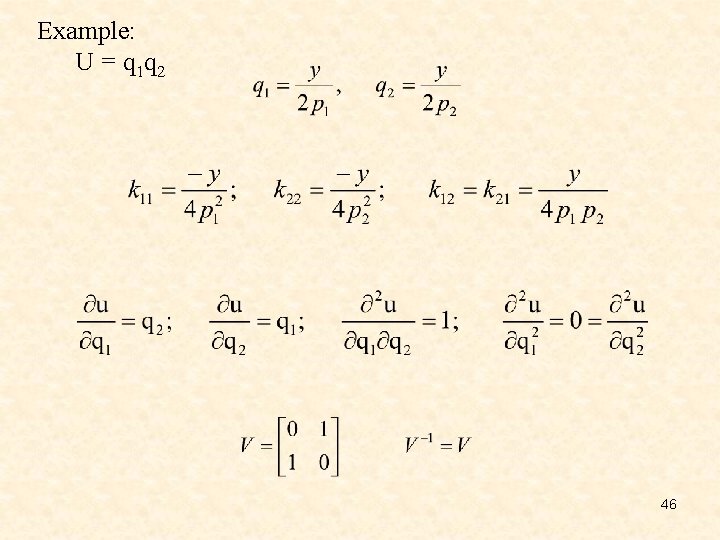
Example: U = q 1 q 2 46

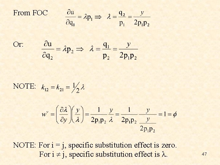
From FOC Or: NOTE: For i = j, specific substitution effect is zero. For i j, specific substitution effect is λ. 47

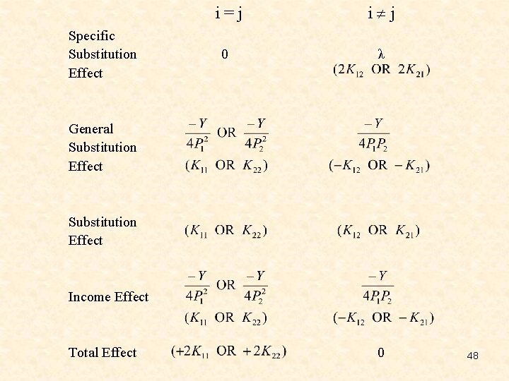
Specific Substitution Effect i=j i j 0 λ General Substitution Effect Income Effect Total Effect 0 48

Show K negative semi-definite Show negative semi-negative 49

Show negative semi-negative, cont. 50

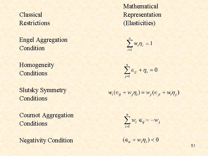
Classical Restrictions Mathematical Representation (Elasticities) Engel Aggregation Condition Homogeneity Conditions Slutsky Symmetry Conditions Cournot Aggregation Conditions Negativity Condition 51

Each of the general restrictions defines an exact set of relationships connecting income and price slopes which any complete set of demand functions must posses if it is derivable from the maximization of any utility function. Under any of the representations, from the viewpoint of applied econometric analysis, the force of the classical theory amounts to a reduction in the dimension of the parameter space in a complete set of demand functions. Of course, the economics of parameterization are not costless. All dynamic considerations are ignored, as are possible feedback from demand to prices and income. 52

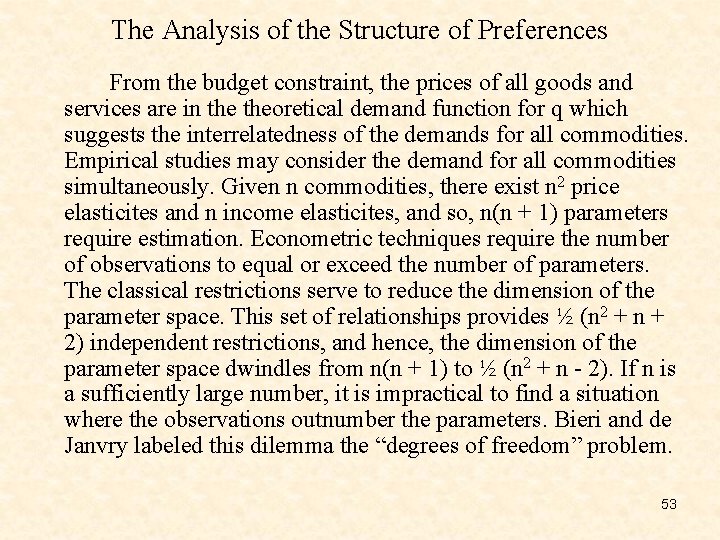
The Analysis of the Structure of Preferences From the budget constraint, the prices of all goods and services are in theoretical demand function for q which suggests the interrelatedness of the demands for all commodities. Empirical studies may consider the demand for all commodities simultaneously. Given n commodities, there exist n 2 price elasticites and n income elasticites, and so, n(n + 1) parameters require estimation. Econometric techniques require the number of observations to equal or exceed the number of parameters. The classical restrictions serve to reduce the dimension of the parameter space. This set of relationships provides ½ (n 2 + n + 2) independent restrictions, and hence, the dimension of the parameter space dwindles from n(n + 1) to ½ (n 2 + n - 2). If n is a sufficiently large number, it is impractical to find a situation where the observations outnumber the parameters. Bieri and de Janvry labeled this dilemma the “degrees of freedom” problem. 53

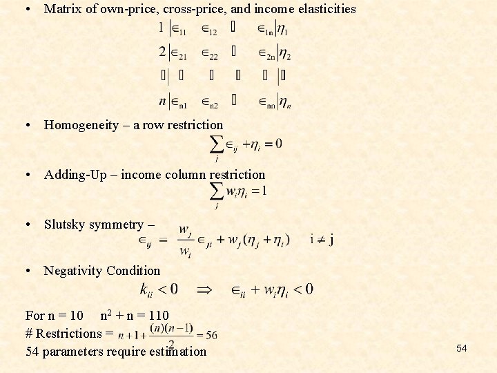
• Matrix of own-price, cross-price, and income elasticities • Homogeneity – a row restriction • Adding-Up – income column restriction • Slutsky symmetry – • Negativity Condition For n = 10 n 2 + n = 110 # Restrictions = 54 parameters require estimation 54

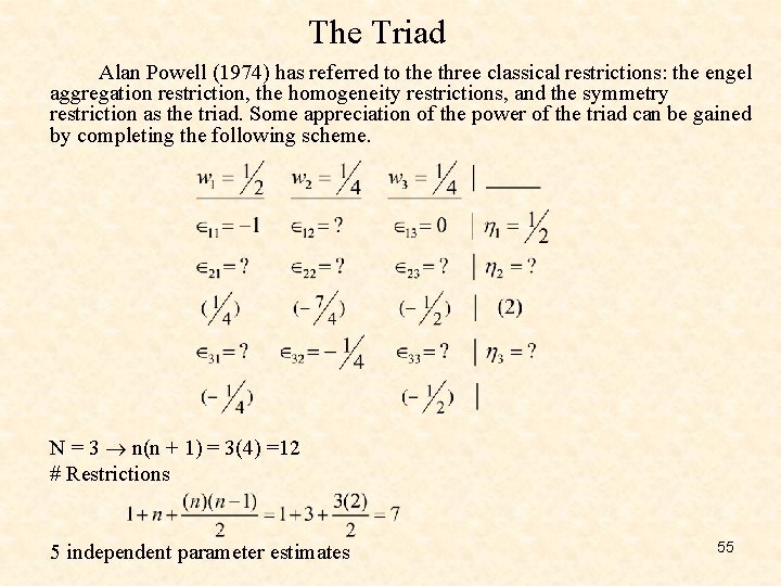
The Triad Alan Powell (1974) has referred to the three classical restrictions: the engel aggregation restriction, the homogeneity restrictions, and the symmetry restriction as the triad. Some appreciation of the power of the triad can be gained by completing the following scheme. N = 3 n(n + 1) = 3(4) =12 # Restrictions 5 independent parameter estimates 55

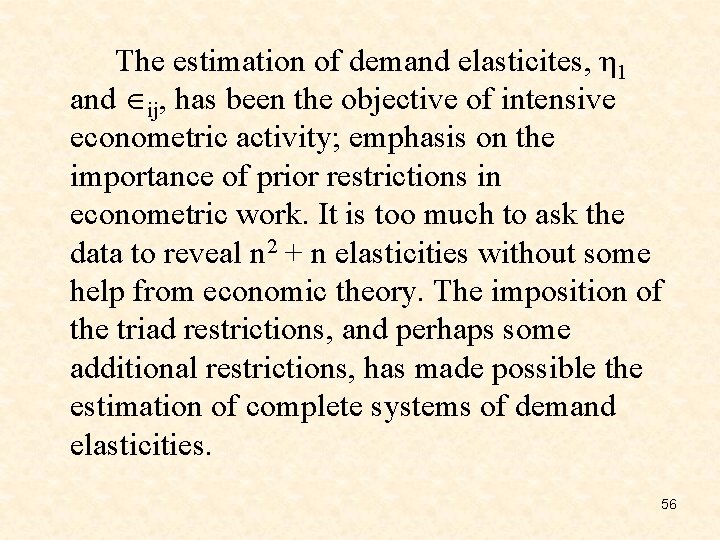
The estimation of demand elasticites, η 1 and ij, has been the objective of intensive econometric activity; emphasis on the importance of prior restrictions in econometric work. It is too much to ask the data to reveal n 2 + n elasticities without some help from economic theory. The imposition of the triad restrictions, and perhaps some additional restrictions, has made possible the estimation of complete systems of demand elasticities. 56

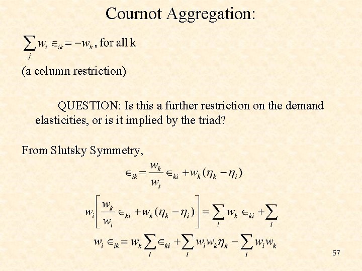
Cournot Aggregation: (a column restriction) QUESTION: Is this a further restriction on the demand elasticities, or is it implied by the triad? From Slutsky Symmetry, 57

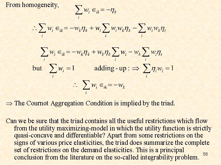
From homogeneity, Þ The Cournot Aggregation Condition is implied by the triad. Can we be sure that the triad contains all the useful restrictions which flow from the utility maximizing-model in which the utility function is strictly quasi-concave and differentiable? Apart from some restrictions on the signs of various price elasticities, the triad does summarize the complete set of restrictions on the demand elasticities. This is a principal 58 conclusion from the literature on the so-called integrability problem.

Several approaches to a solution to the degrees of freedom problem exist: (1) gainfully employ single commodity or sector models under the explicit assumption that omitted factors have zero effects; (2) increase the number of available observations, for instance, to combine time-series and cross-sectional data; (3) aggregate commodities with the use of the Leontief-Hicks composite commodity theorem – commodities whose relative prices do not change are, in effect, a single commodity for the purposes of theory; and (4) recognize the inter-relationships among all commodities and make a number of assumptions regarding the interaction of commodities and the nature of utility functions. This last approach forms the foundation of additive preferences, almost additive preferences, and separability conditions – the modern theory of consumer demand. 59

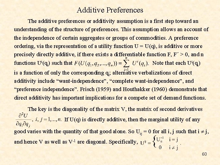
Additive Preferences The additive preferences or additivity assumption is a first step toward an understanding of the structure of preferences. This assumption allows an account of the independence of certain aggregates or groups of commodities. A preference ordering, via the representation of a utility function U = U(q), is additive or more precisely directly additive, if there exists a differentiable function F, F΄ > 0, and n functions Ui(qi) such that Note that each Ui(qi) is a function of only the corresponding qi; alternative verbalizations of direct additivity include “want-independence”, “complete want-independence”, and “preference independence”. Frisch (1959) and Houthakker (1960) demonstrate that direct additivity has important implications for a compete set of demand functions. The key is the diagonality of the matrix V, the matrix of second derivatives If U(q) is directly additive, then the marginal utility of any good varies with the quantity of that good alone. So Uij = 0 for all i, j such that i j, and hence V as well as V-1 are diagonal. Specifically, 60

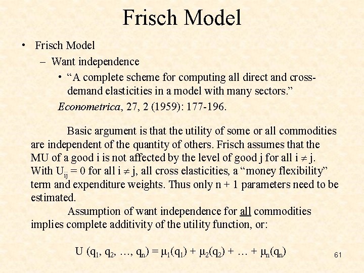
Frisch Model • Frisch Model – Want independence • “A complete scheme for computing all direct and crossdemand elasticities in a model with many sectors. ” Econometrica, 27, 2 (1959): 177 -196. Basic argument is that the utility of some or all commodities are independent of the quantity of others. Frisch assumes that the MU of a good i is not affected by the level of good j for all i j. With Uij = 0 for all i j, all cross elasticities, a “money flexibility” term and expenditure weights. Thus only n + 1 parameters need to be estimated. Assumption of want independence for all commodities implies complete additivity of the utility function, or: U (q 1, q 2, …, qn) = μ 1(q 1) + μ 2(q 2) + … + μn(qn) 61

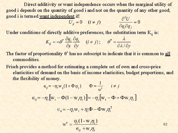
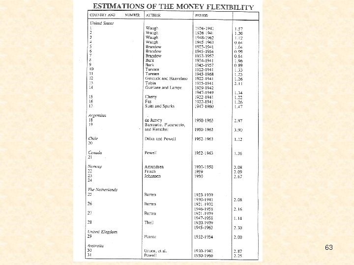
Direct additivity or want independence occurs when the marginal utility of good i depends on the quantity of good i and not on the quantity of any other good; good i is termed want independent if: Under conditions of directly additive preferences, the substitution term Kij is: The factor of proportionality θ* has no subscript to indicate that it is common to all commodities. Frisch provides a method for estimating a complete set of own and cross-price elasticities of demand on the basis of income elasticities, budget proportions, and the flexibility of money. 62

63

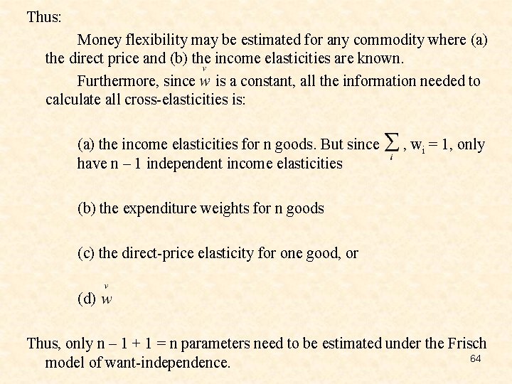
Thus: Money flexibility may be estimated for any commodity where (a) the direct price and (b) the income elasticities are known. Furthermore, since is a constant, all the information needed to calculate all cross-elasticities is: (a) the income elasticities for n goods. But since have n – 1 independent income elasticities , wi = 1, only (b) the expenditure weights for n goods (c) the direct-price elasticity for one good, or (d) Thus, only n – 1 + 1 = n parameters need to be estimated under the Frisch 64 model of want-independence.

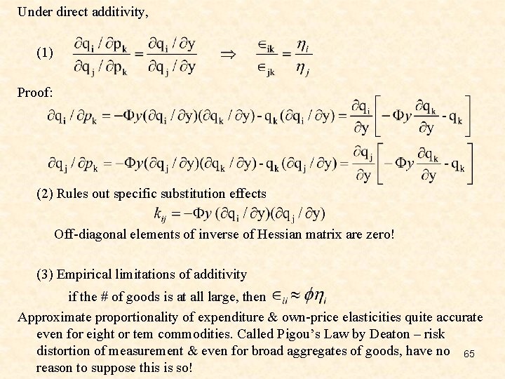
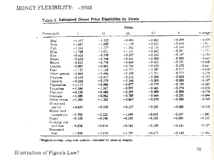
Under direct additivity, (1) Proof: (2) Rules out specific substitution effects Off-diagonal elements of inverse of Hessian matrix are zero! (3) Empirical limitations of additivity if the # of goods is at all large, then Approximate proportionality of expenditure & own-price elasticities quite accurate even for eight or tem commodities. Called Pigou’s Law by Deaton – risk distortion of measurement & even for broad aggregates of goods, have no 65 reason to suppose this is so!

In short, a directly additive utility function leads to substantial economies in the parameterization of a complete set of demand functions beyond those obtainable from the classical theory. Within this framework, only n parameters require estimation. However, these economies are costless. Direct additivity rules out the possibility of specific substitution effects, the possibility of inferior goods, and the possibility of complementary goods. In light of these restrictions, direct additivity may be a plausible specification when goods are broad aggregates. For the case where a fine classification of goods exists, this specification is not tenable. In the latter case, specific substitution effects, complementary goods, and inferior foods may be present. 66

Practical Applications of Frisch Method (1) Ayanian, R. , “A Comparison of Barten’s Estimated Demand Elasticities with Those Obtained using Frisch’s Method, ” Econometrica, 37, 1 (January 1969): 79 -94. Compared Frisch’s method of want independence with Barten’s method which allowed 22 non-zero Uij’s for same data bases. (2) Pinstrup-Anderson, et al. 67

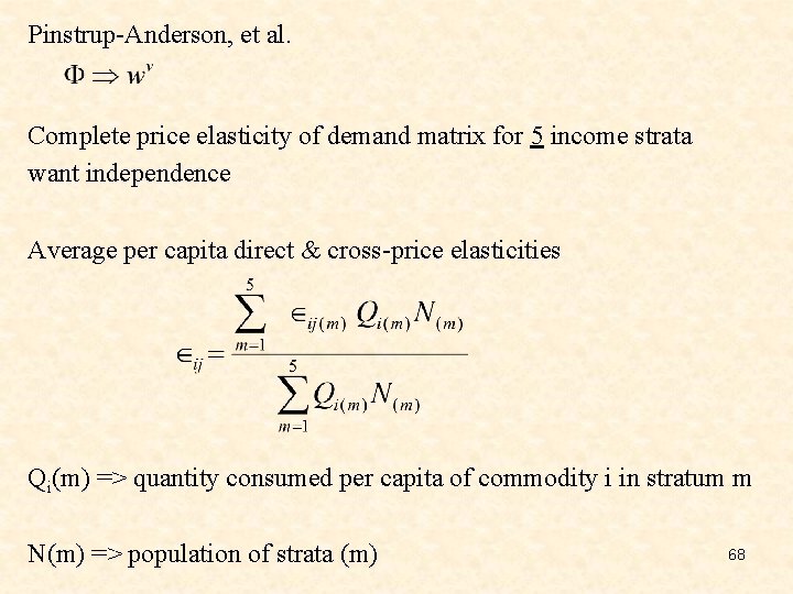
Pinstrup-Anderson, et al. Complete price elasticity of demand matrix for 5 income strata want independence Average per capita direct & cross-price elasticities Qi(m) => quantity consumed per capita of commodity i in stratum m N(m) => population of strata (m) 68

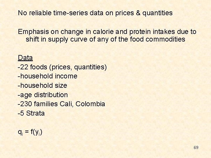
No reliable time-series data on prices & quantities Emphasis on change in calorie and protein intakes due to shift in supply curve of any of the food commodities Data -22 foods (prices, quantities) -household income -household size -age distribution -230 families Cali, Colombia -5 Strata qi = f(yi) 69

70

The Separability Approach (Stimulated by pioneering paper of Strotz) The approaches of Frisch, Houthakker, and Barten assume additivity and almost additivity of the utility function, and hence, very little interaction among commodities in the utility function. A concept of separability evolves from Strotz’s (1957) utility tree representation. There has been a tendency in recent years for some economists to consider restrictions in the form of various separability conditions on the consumer’s utility function. Separability is a relative concept whose frame of reference is some partition of the complete set of n commodities into S mutually exclusive and exhaustive subsets. In general, the separability conditions, which are exact properties of the utility function, require the marginal rates of substitution for certain pairs of commodities to be functionally independent of the quantities of certain other commodities. Restrictions such as these reduce the number of parameters that enter into the gamily of demand functions and in short, make estimation of the entire parameter space more feasible. In general, three types of separability definitions are in existence – weak separability, strong separability, and Pearce separability. Each of these intuitively tenable 71 relationships warrants consideration.

Separability Approach Concept – Classical approach by Frisch and Barten assumes additivity and almost additivity of the utility function, i. e. , very little interaction among commodities in the utility function. Different approach is the concept of separability evolving from the “utility tree” concept developed by Strotz. (Strotz, R. H. , “The Empirical Implications of a Utility Tree. ” Econometrica, 25, 2 (1957): 269 -80. ) Basic idea is that the elements belonging to the commodity bundle may be partitioned into different groups. Budget allocation, then, is a step-wise procedure whereby the consumer first allocates his total budget among groups and then the amounts allocated to the groups are allocated among individual commodities within a group. 72

General Concept of Separability of commodities within a utility function in general assumes that the ratio of marginal utilities of a pair of commodities i and j is unaffected by the level of consumption of a third commodity k. That is; it is assumed that: holds for at least some goods. We note here that Frisch’s want independence (additivity) assumes that the marginal utility of every good is independent of the quantity consumed of all other goods. Various types of separability assume only that the marginal utilities are changed equally because of a change in the consumption of the kth commodity. Given various assumptions, we can define three types of separability. 73

Separable Utility Functions Under what conditions may the arguments of the utility functions be aggregated? Intuitively wish to partition the consumption set into subsets which would include commodities that are closer substitutes or complements to each other than members of other subsets U = F(A, B) where A = f. A(q 1, q 2) B = f. B(q 3, q 4, q 5) Want the value of U to be the same w/ or w/out the grouping, i. e. whether U is expressed as a function of all elementary variables or as a function of the groups. U (food, housing, automobiles) U (food, durable goods) 74

Necessary and Sufficient condition for a function to be separablethe marginal rate of substitution between any two variables (belonging to the same group) be independent of the value of any variable in any other group (Leontief’s theorem) weak separability strong separability, pearce separability Weak separability prerequisite for the consistency of the two-stage maximization procedure discussed by Strotz. Procedure in two steps: (1) Optimal allocation of income among broad commodity groups –a budget allocation (say yr) to each “branch” of the utility function. (2) Optimal spending of each budget allotment in its branch, with no further reference to purchases in other branches. Tantamount to maximizing each branch utility function subject to the budget constraint Conditional Demand Functions 75

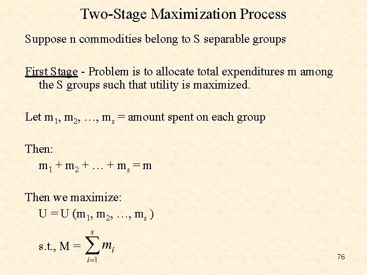
Two-Stage Maximization Process Suppose n commodities belong to S separable groups First Stage - Problem is to allocate total expenditures m among the S groups such that utility is maximized. Let m 1, m 2, …, ms = amount spent on each group Then: m 1 + m 2 + … + m s = m Then we maximize: U = U (m 1, m 2, …, ms ) s. t. , M = 76

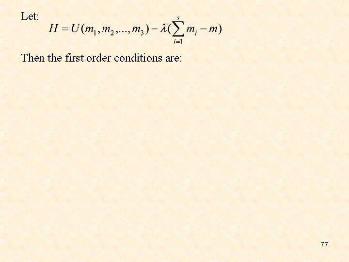
Let: Then the first order conditions are: 77

Implications of Separability Additional restrictions on Kij Additional restrictions on the number of variables that appear as arguments in the demand functions. The demand for a commodity in a branch can be expressed as a function of the prices in and the budget allotment to that branch. The quantities demanded in one branch are NOT independent of the prices of commodities in other branches or of total expenditures. Total income and the prices of goods outside the branch enter the demand functions for goods in the branch only through their effect on yr, the budget allotment to that branch, we can ignore the prices of goods outside the branch. 78

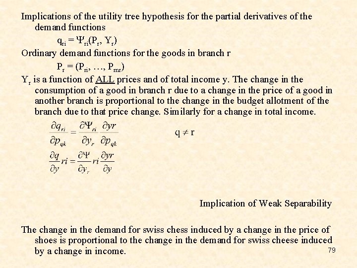
Implications of the utility tree hypothesis for the partial derivatives of the demand functions qri = ri(Pr, Yr) Ordinary demand functions for the goods in branch r Pr = (Pri, …, Prnr) Yr is a function of ALL prices and of total income y. The change in the consumption of a good in branch r due to a change in the price of a good in another branch is proportional to the change in the budget allotment of the branch due to that price change. Similarly for a change in total income. Implication of Weak Separability The change in the demand for swiss chess induced by a change in the price of shoes is proportional to the change in the demand for swiss cheese induced 79 by a change in income.