Inventory Management Independent vs dependent demand n Independent


 B(4) D(2) E(1) D(3) F(2) Independent demand is")


 n Assumptions of the model: n n n n Demand")
 Average inventory level = Q/2")
 cost Total cost")

 TC = S ∙ (D/Q) + H ∙ (Q/2) +")

 point When to start the ordering process? n It depends on")


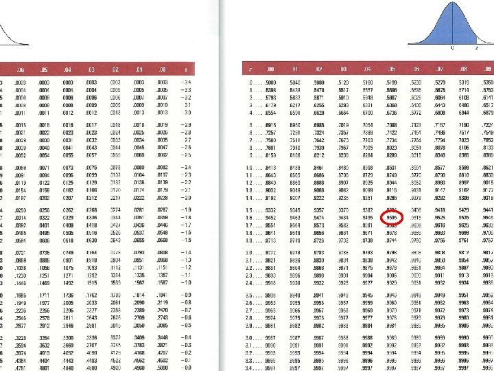
 stock b=z∙σ where z = safety factor from the (normal) distribution σ")


 is given, at")

- Slides: 31
Inventory Management
Independent vs. dependent demand n Independent demand: Influenced only by market conditions n Independent from operations n Example: finished goods n n Dependent demand: Related to the demand for another item with independent demand n Example: product components, raw materials, labour n
Independent Demand Dependent Demand A C(2) B(4) D(2) E(1) D(3) F(2) Independent demand is uncertain. Dependent demand is certain.
Inventory management A subsystem of logistics n Inventory: n a stock of materials or other goods to facilitate production or to satisfy customer demand n a stock or store of goods n n Main decisions: Which items should be carried in stock? n How much should be ordered? n When should an order be placed? n
The need to hold stocks 1 n n Buffer between Supply and Demand To keep down production costs: n n n To achieve low unit costs, production have to run as long as possible (setting up machines is tend to be costly) To decouple operations To take account of variable supply (lead) times: safety stock to cover delivery delays from suppliers To minimize buying costs associated with raising an order To accommodate variations (on the short run) in demand (to avoid stock-outs) To account for seasonal fluctuations: n n There are products popular only in peak times There are goods produced only at a certain time of the year
Adaptation o the fluctuation of demand with building up stocks DEMAND Inventory accumulation CAPACITY Inventory reduction
The need to hold stocks 2 n n n To take advantage of quantity discounts (buying in bulk) To allow for price fluctuations/speculation: to buy large quantities when a good is cheaper To help production and distribution operations run smoothly: to increase the independence of these activities. n n n Work-in-progress: facilitating production process by providing semi-finished stocks between different processes To provide immediate service for customers To minimize production delays caused by lack of spare parts (for maintenance, breakdowns)
Types of Stock-holding/Inventory n n n raw material, component and packaging stock in-process stocks (work-in-progress; WIP) finished products (finished goods inventory; FGI) pipeline stocks: held in the distribution chain general stores: contains a mixture of products to support spare parts for production: n n Consumables (nuts, bolts, etc. ) Rotables and repairables
An alternative typology of stocks working stock: reflects the normal demand n cycle stock: follows the production (or demand) cycles n n seasonal stock: goods stockpiled before peaks safety stock: to cover unexpected fluctuations in demand n speculative stock: built up on expectations n
Inventory cost n n n Item cost: the cost of buying or producing inventory items Ordering cost: does not depend on the number of items ordered. Form typing the order to transportation and receiving costs. Holding (carrying) cost: n n Capital cost: the opportunity cost of tying up capital Storage cost: space, insurance, tax Cost of obsolescence, deterioration and loss Stock-out cost: economic consequences of running out of stock (lost profit and/or goodwill)
Evaluating stocks: the ABC analysis
Data Capture n Techniques and error rates n n n Written entry – 25, 000 in 3, 000 Keyboard entry – 10, 000 in 3, 000 Optical character recognition (OCR) – 100 in 3, 000 n n n labels that are both machine- and human-readable for example: license plates Bar code (code 39) – 1 in 3, 000 n n n (Rushton et al. 2006) fast, accurate and fairly robust reliable and cheap technique Transponders (radio frequency tags) – 1 in 30, 000 n n n a tag (microchip + antenna) affixed to the goods or container receiver antenna reader host station that relays the data to the server can be passive or active
Inventory models
Economic Order Quantity (EOQ) n Assumptions of the model: n n n n Demand rate is constant, recurring and known The lead time (from order placement and order delivery) is constant and known No stockouts are allowed Goods are ordered and produced in lots, and the lot is placed into inventory all at one time Unit item cost is constant, carrying cost is linear function of average inventory level Ordering cost is independent of the number of items in a lot The item is a single product (no interaction with other products)
The ‘SAW-TOOTH’ Inventory level Order inteval Order quantity (Q) Average inventory level = Q/2 Time
Total cost of inventory (trade-off between ordering frequency and inventory level) cost Total cost Holding cost (H ∙ Q/2) Minimum cost Ordering cost (S ∙ D/Q) EOQ lot size
Calculating the total cost of inventory n Let… n n n S be the ordering cost (setup cost) per oder D be demanded items per planning period H be the stock holding cost per unit n n n H=i∙C, where C is the unit cost of an item, and i is the carrying rate P be the market price of the item demanded Q be the ordered quantity per order (= lot) TC = S ∙ (D/Q) + H ∙ (Q/2) + P ∙ D (D/Q) is the number of orders period (Q/2) is the average inventory level in this model
The minimum cost (EOQ) TC = S ∙ (D/Q) + H ∙ (Q/2) + P ∙ D n б. TC/б. Q = 0 n 0 = – S ∙ (D/Q 2) + H/2 n H/2 = S ∙ (D/Q 2) n Q 2 = (2 ∙ S ∙ D)/H n EOQ = √ (2 ∙ S ∙ D)/H n
Example D = 1000 units per year S = 100 euro per order H = 20 euro per unit per year Find the economic order quantity! (we assume a saw-tooth model) EOQ = √ (2 ∙ 1, 000 units ∙ 100 euro)/20 euro/unit EOQ = √ 10, 000 units = 100 units 2
Reordering (or replenishment) point When to start the ordering process? n It depends on the… n n Stock position: stock on-hand (+ stock on-order) n in a simple saw-tooth model it is Q, n in some cases, there can be an initial stock, that is different from Q. lead time (L): the time interval from setting up order to the start of using up the ordered stock n Average demand per day (d) n n ROP = d ∙ L
Examples n n n n Q = 200 tons d = 10 tons per day L = 8 days ROP = ? ROP = 10 ∙ 8 = 80 tons Q = 400 tons d = 16 tons per day L =20 days ROP = ? ROP = 16 ∙ 20 = 320 tons
Example on both EOQ and R D = 2, 000 tons S = 100 euros per order H = 25 euros per unit per year L = 12 days N = 250 days Calculate the following: EOQ d ROP EOQ = √ (2 ∙ 2, 000 ts ∙ 100 euro)/25 euro/ts = 126, 49 tons d = 2, 000 ts/250 ds = 8 ts/ds ROP = 8 ∙ 12 = 96 tons
The SAW-TOOTH with safety stock Inventory level Continuous demand Order quantity b Safety stock or buffer stock Time
Buffer (safety) stock b=z∙σ where z = safety factor from the (normal) distribution σ = sandard deviation of demand over lead time Let z be 1, 65 (95%), and the standard deviation of demand is 200 units/lead time. b = 1, 65 ∙ 200 units = 330 units
When to order, when there is a buffer stock? ROP = d * L + b If Q = 60 tons, L = 2 days, b = 10 tons, D = 300 tons, N = 100 days, then ROP = ? ROP = 2 * 3 + 10 = 16 tons
Example n n n Lead time = 10 days Average demand over lead time: 300 tons Standard deviation over lead time: 20 tons Accepted risk level: 5% Safety stock = ? Reorder quantity = ? b = z * σ = 1, 65 * 20 = 33 tons n ROP = 300 + 33 = 333 tons n
Examples n n n n n Q 0 = 600 tons Q = 200 tons d = 10 tons per day L = 8 days b = 33 tons ROP = 8 * 10 + 33 = 113 Q 0 = Q = 400 tons d = 16 tons per day L =20 days b = 66 tons ROP = 386
Alternative models 1 Periodic review system: Stock level is examined at regular intervals n Size of the order depends on the quantity on stock. it should bring the inventory to a predetermined level n Stock on hand Q Q Q time T L L L T T
Alternative models 2 Fixed-order-quantity system: A predetermined stock level (reorder point) is given, at which the replenishement order will be placed n The order quantity is constant n Stock on hand Q Q R L L L
Some more examples Calculate ROP, and EOQ, if… 1. 2. 3. L = 2 days, b = 12 tons, D = 300 tons, N = 100 days, S = 50 euro, H = 20 euro/tons/year L = 12 days, b = 20 tons, D = 1300 tons, N = 80 days, S = 10 euro, H = 25 euro/ton/year D = 1000 units, N = 500 days, S = 110 euro, H = 100 euro/unit/year, L = 20 days, b = 50 tons