Rendering the Teapot 1 Utah Teapot 2 Angel

Rendering the Teapot 1

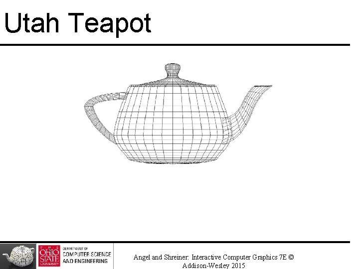
Utah Teapot 2 Angel and Shreiner: Interactive Computer Graphics 7 E © Addison-Wesley 2015

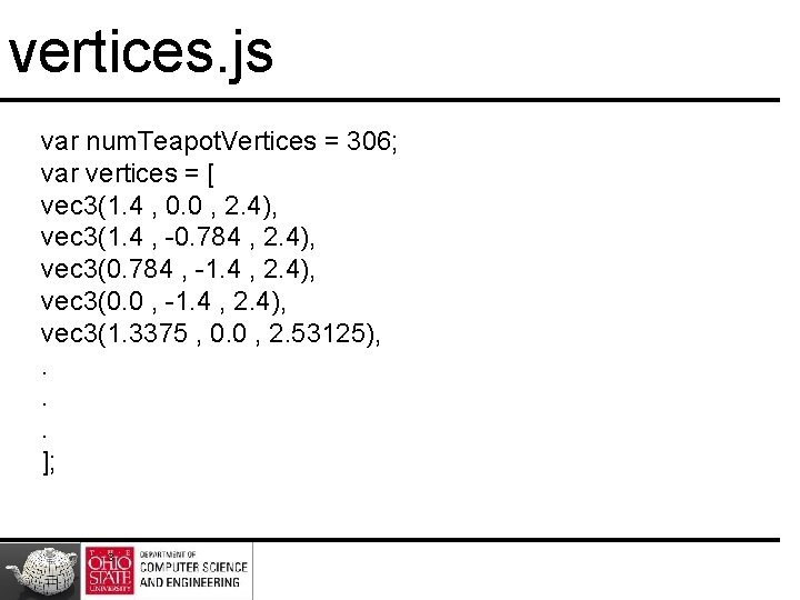
vertices. js var num. Teapot. Vertices = 306; var vertices = [ vec 3(1. 4 , 0. 0 , 2. 4), vec 3(1. 4 , -0. 784 , 2. 4), vec 3(0. 784 , -1. 4 , 2. 4), vec 3(0. 0 , -1. 4 , 2. 4), vec 3(1. 3375 , 0. 0 , 2. 53125), . . . ]; 3

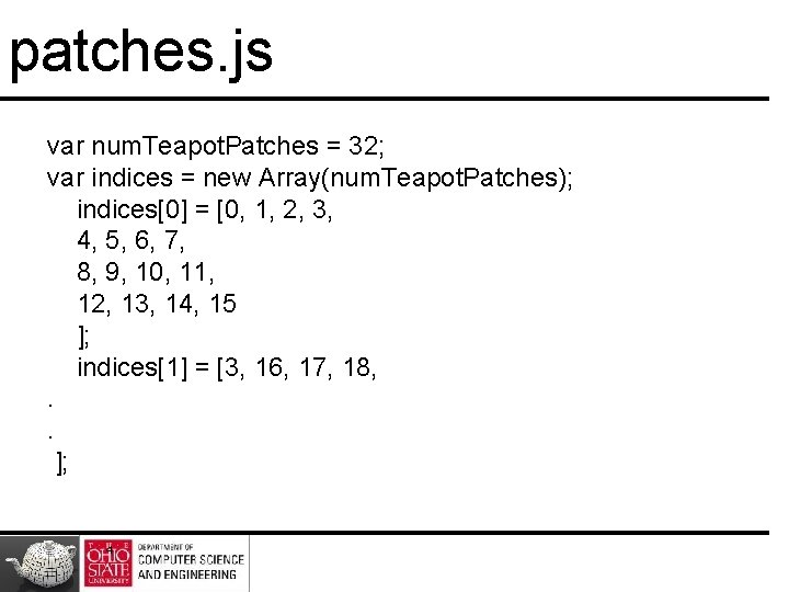
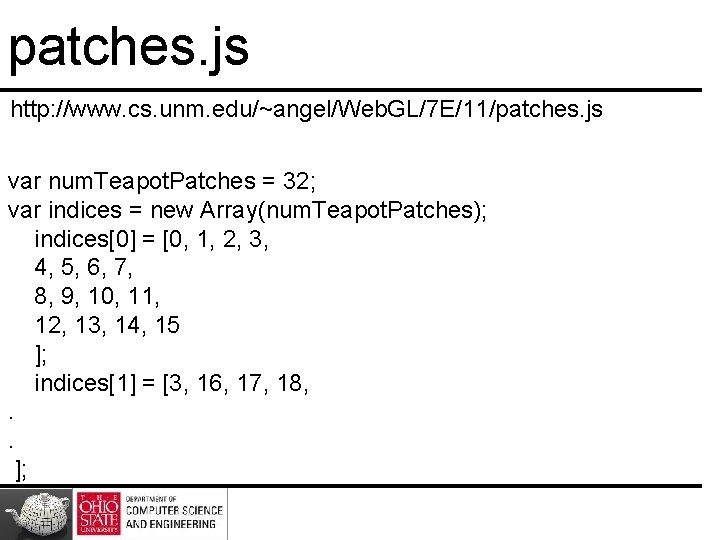
patches. js var num. Teapot. Patches = 32; var indices = new Array(num. Teapot. Patches); indices[0] = [0, 1, 2, 3, 4, 5, 6, 7, 8, 9, 10, 11, 12, 13, 14, 15 ]; indices[1] = [3, 16, 17, 18, . . ]; 4

Evaluation of Polynomials 5

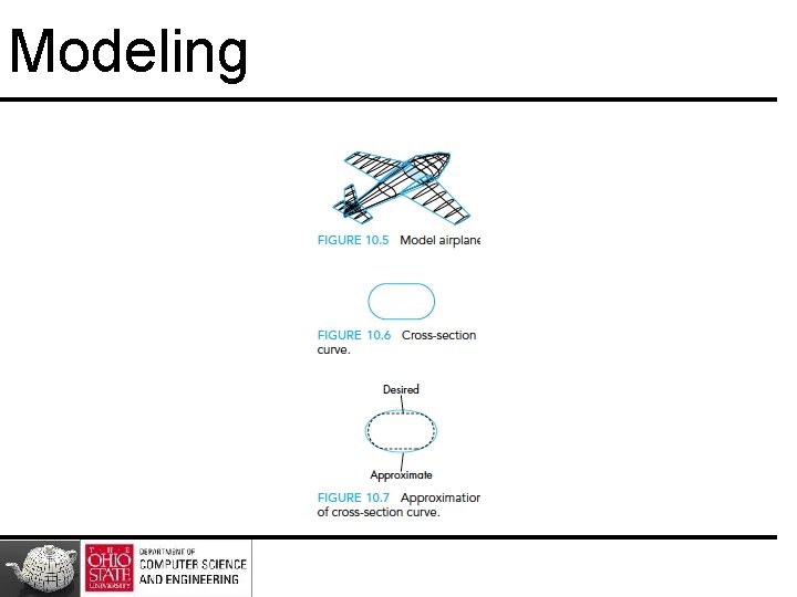
Modeling

Topics • Introduce types of curves and surfaces – Explicit – Implicit – Parametric • Discuss Modeling and Approximations

Escaping Flatland • Lines and flat polygons – Fit well with graphics hardware – Mathematically simple • But world is not flat – Need curves and curved surfaces – At least at the application level – Render them approximately with flat primitives

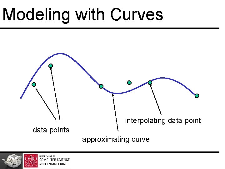
Modeling with Curves interpolating data points approximating curve 9

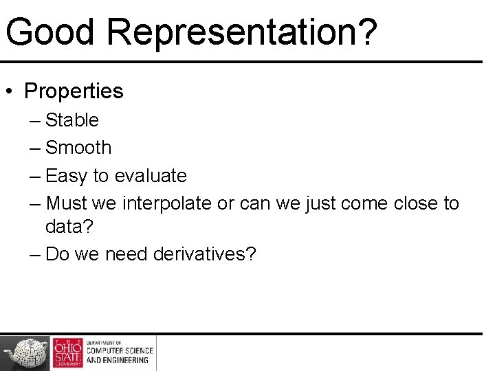
Good Representation? • Properties – Stable – Smooth – Easy to evaluate – Must we interpolate or can we just come close to data? – Do we need derivatives?

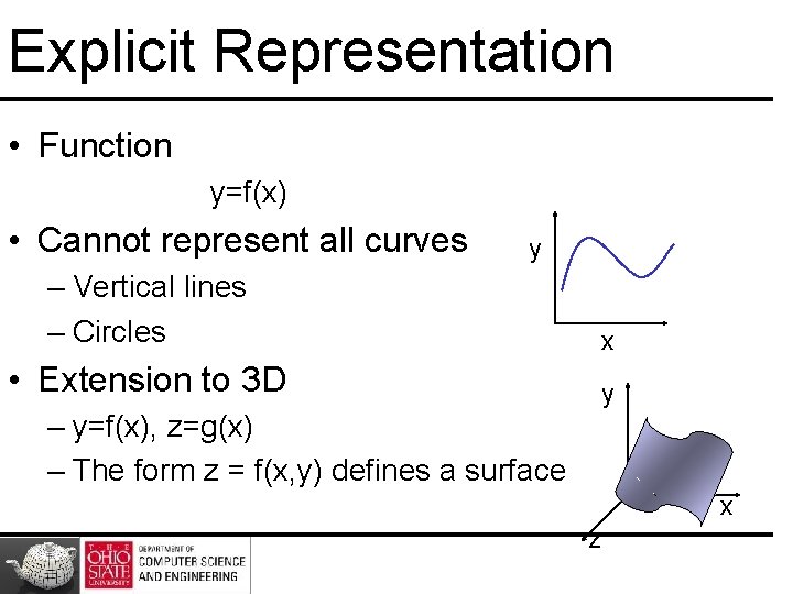
Explicit Representation • Function y=f(x) • Cannot represent all curves y – Vertical lines – Circles x • Extension to 3 D y – y=f(x), z=g(x) – The form z = f(x, y) defines a surface x z

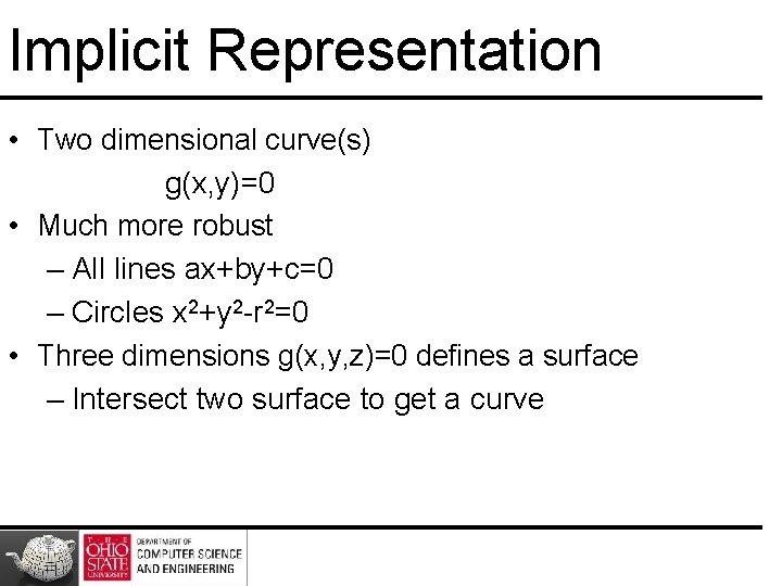
Implicit Representation • Two dimensional curve(s) g(x, y)=0 • Much more robust – All lines ax+by+c=0 – Circles x 2+y 2 -r 2=0 • Three dimensions g(x, y, z)=0 defines a surface – Intersect two surface to get a curve

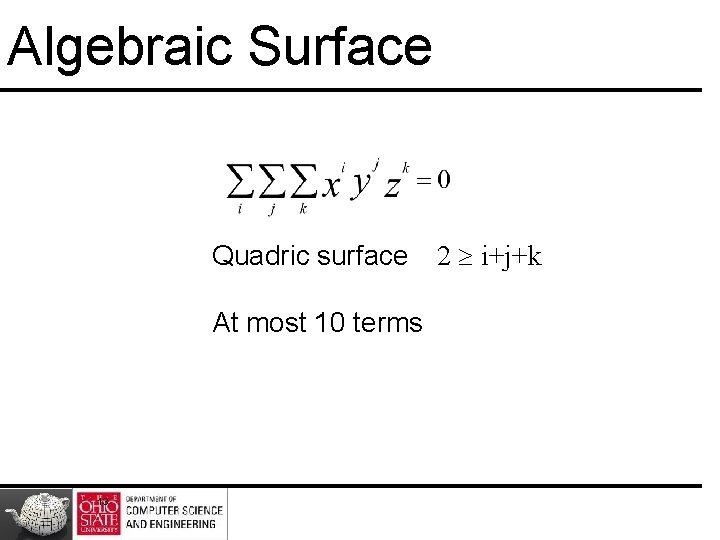
Algebraic Surface Quadric surface At most 10 terms 13 2 i+j+k

Parametric Curves • Separate equation for each spatial variable x=x(u) y=y(u) p(u)=[x(u), y(u), z(u)]T z=z(u) • For umax u umin we trace out a curve in two or three dimensions p(u) p(umax) p(umin) 14

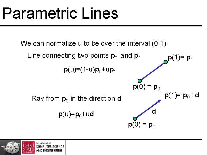
Parametric Lines We can normalize u to be over the interval (0, 1) Line connecting two points p 0 and p 1 p(1)= p 1 p(u)=(1 -u)p 0+up 1 p(0) = p 0 Ray from p 0 in the direction d p(u)=p 0+ud d p(0) = p 0 15 p(1)= p 0 +d

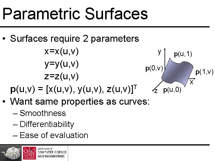
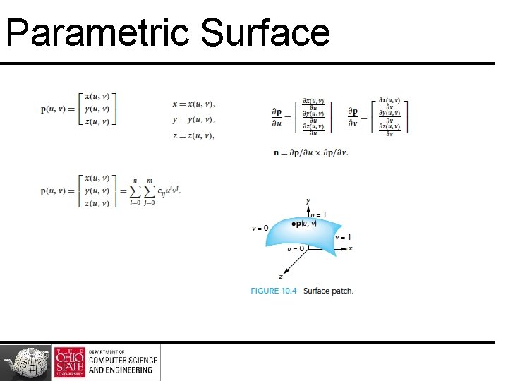
Parametric Surfaces • Surfaces require 2 parameters y x=x(u, v) p(u, 1) y=y(u, v) p(0, v) p(1, v) z=z(u, v) x p(u, v) = [x(u, v), y(u, v), z(u, v)]T z p(u, 0) • Want same properties as curves: – Smoothness – Differentiability – Ease of evaluation 16

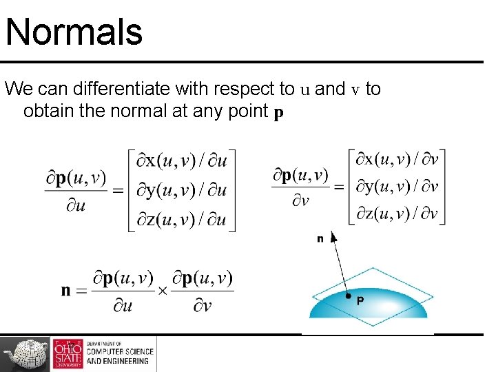
Normals We can differentiate with respect to u and v to obtain the normal at any point p 17

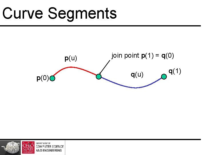
Curve Segments p(u) p(0) 18 join point p(1) = q(0) q(u) q(1)

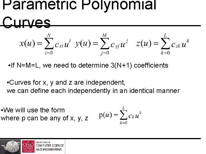
Parametric Polynomial Curves • If N=M=L, we need to determine 3(N+1) coefficients • Curves for x, y and z are independent, we can define each independently in an identical manner • We will use the form where p can be any of x, y, z 19

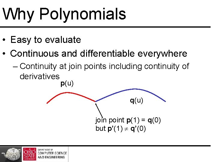
Why Polynomials • Easy to evaluate • Continuous and differentiable everywhere – Continuity at join points including continuity of derivatives p(u) q(u) join point p(1) = q(0) but p’(1) q’(0)

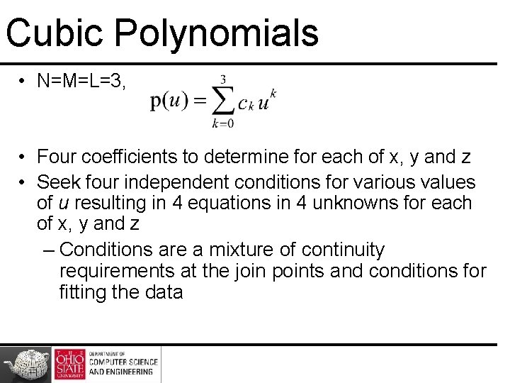
Cubic Polynomials • N=M=L=3, • Four coefficients to determine for each of x, y and z • Seek four independent conditions for various values of u resulting in 4 equations in 4 unknowns for each of x, y and z – Conditions are a mixture of continuity requirements at the join points and conditions for fitting the data

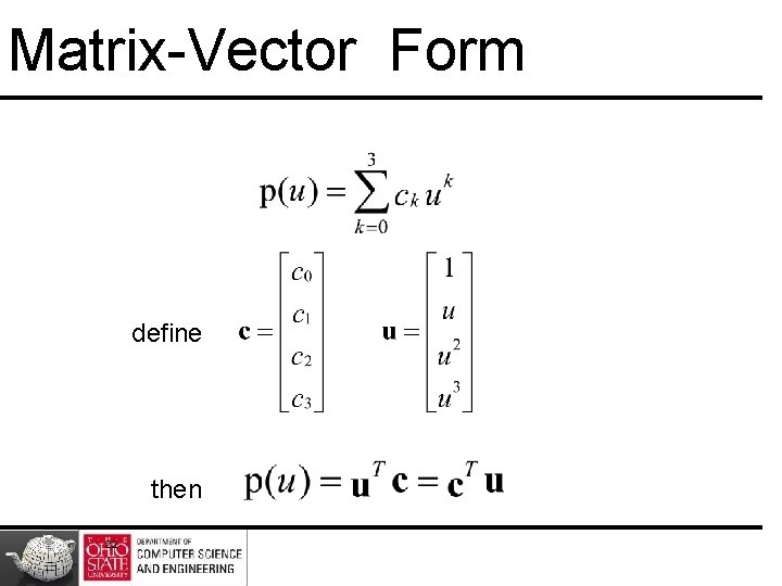
Matrix-Vector Form define then 22

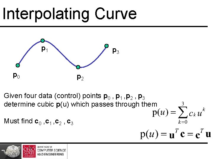
Interpolating Curve p 1 p 0 p 3 p 2 Given four data (control) points p 0 , p 1 , p 2 , p 3 determine cubic p(u) which passes through them Must find c 0 , c 1 , c 2 , c 3 23

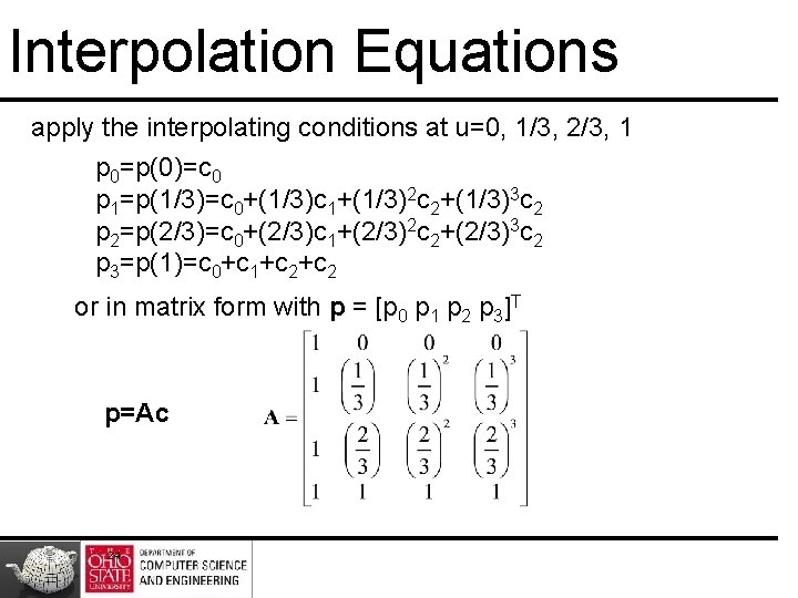
Interpolation Equations apply the interpolating conditions at u=0, 1/3, 2/3, 1 p 0=p(0)=c 0 p 1=p(1/3)=c 0+(1/3)c 1+(1/3)2 c 2+(1/3)3 c 2 p 2=p(2/3)=c 0+(2/3)c 1+(2/3)2 c 2+(2/3)3 c 2 p 3=p(1)=c 0+c 1+c 2 or in matrix form with p = [p 0 p 1 p 2 p 3]T p=Ac 24

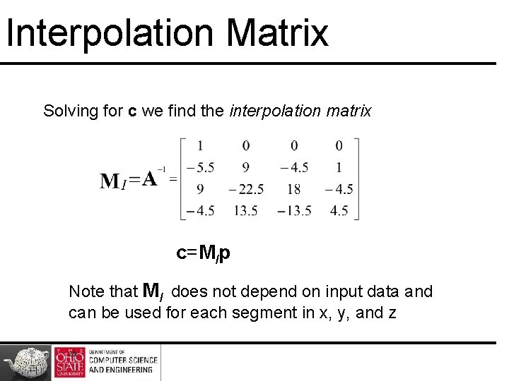
Interpolation Matrix Solving for c we find the interpolation matrix c=MIp Note that MI does not depend on input data and can be used for each segment in x, y, and z 25

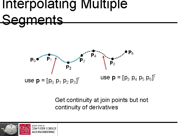
Interpolating Multiple Segments use p = [p 0 p 1 p 2 p 3 ]T use p = [p 3 p 4 p 5 p 6]T Get continuity at join points but not continuity of derivatives 26

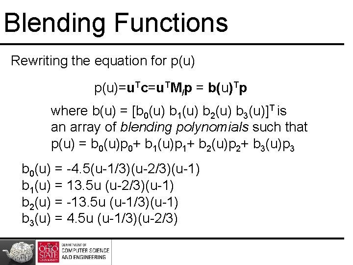
Blending Functions Rewriting the equation for p(u)=u. Tc=u. TMIp = b(u)Tp where b(u) = [b 0(u) b 1(u) b 2(u) b 3(u)]T is an array of blending polynomials such that p(u) = b 0(u)p 0+ b 1(u)p 1+ b 2(u)p 2+ b 3(u)p 3 b 0(u) = -4. 5(u-1/3)(u-2/3)(u-1) b 1(u) = 13. 5 u (u-2/3)(u-1) b 2(u) = -13. 5 u (u-1/3)(u-1) b 3(u) = 4. 5 u (u-1/3)(u-2/3) 27

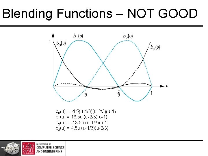
Blending Functions – NOT GOOD b 0(u) = -4. 5(u-1/3)(u-2/3)(u-1) b 1(u) = 13. 5 u (u-2/3)(u-1) b 2(u) = -13. 5 u (u-1/3)(u-1) b 3(u) = 4. 5 u (u-1/3)(u-2/3) 28

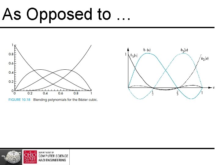
As Opposed to …

Parametric Surface

Cubic Polynomial Surfaces p(u, v)=[x(u, v), y(u, v), z(u, v)]T where p is any of x, y or z Need 48 coefficients ( 3 independent sets of 16) to determine a surface patch 31

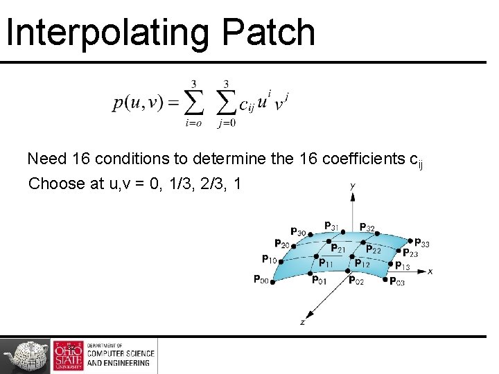
Interpolating Patch Need 16 conditions to determine the 16 coefficients cij Choose at u, v = 0, 1/3, 2/3, 1 32

Matrix Form Define v = [1 v v 2 v 3]T C = [cij] P = [pij] p(u, v) = u. TCv If we observe that for constant u (v), we obtain interpolating curve in v (u), we can show C=MIPMI p(u, v) = u. TMIPMITv 33

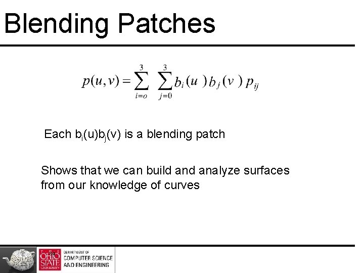
Blending Patches Each bi(u)bj(v) is a blending patch Shows that we can build analyze surfaces from our knowledge of curves 34

Bezier and Spline Curves and Surfaces

Bezier

Bezier Surface Patches

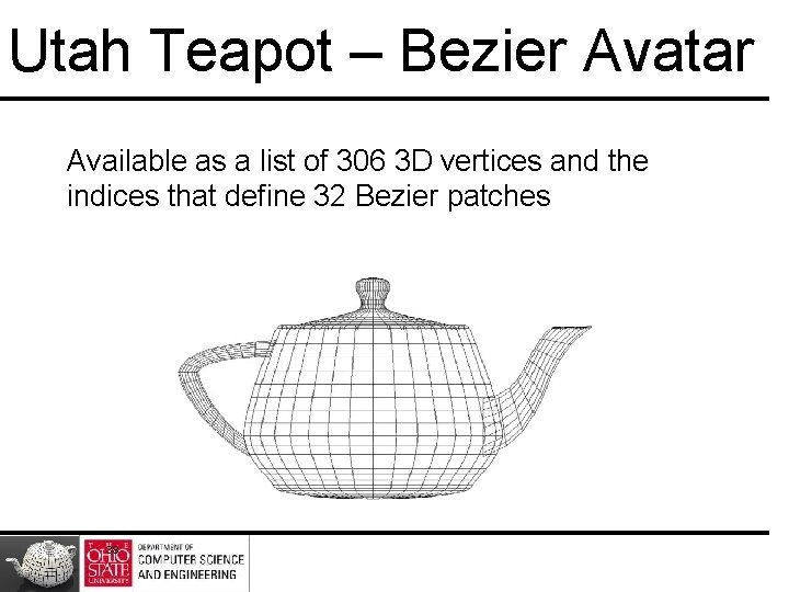
Utah Teapot – Bezier Avatar Available as a list of 306 3 D vertices and the indices that define 32 Bezier patches 38

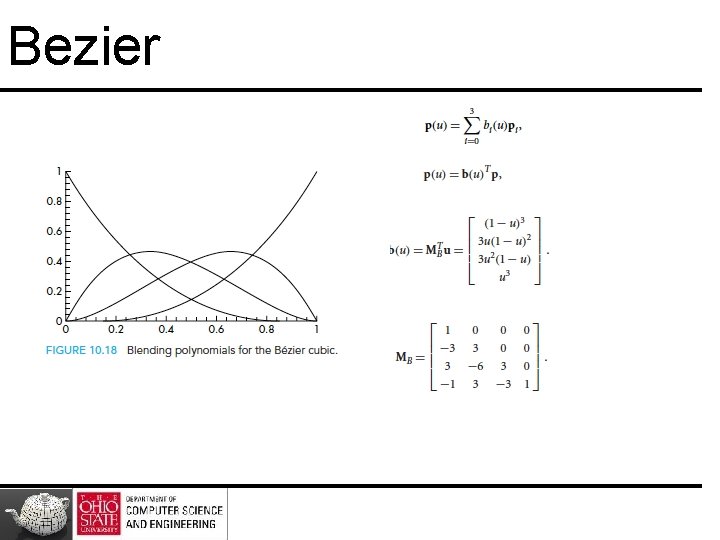
Bezier • Do not usually have derivative data • Bezier suggested using the same 4 data points as with the cubic interpolating curve to approximate the derivatives 39

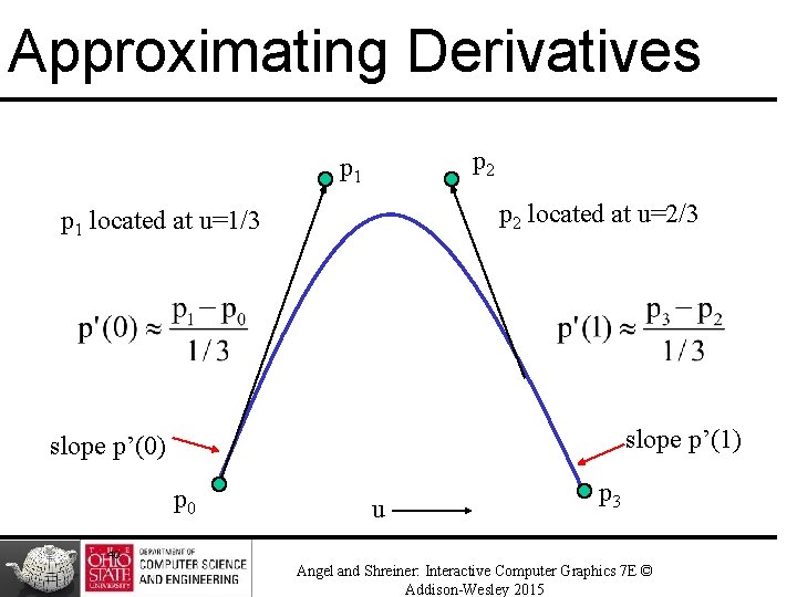
Approximating Derivatives p 2 p 1 p 2 located at u=2/3 p 1 located at u=1/3 slope p’(1) slope p’(0) p 0 u p 3 40 Angel and Shreiner: Interactive Computer Graphics 7 E © Addison-Wesley 2015

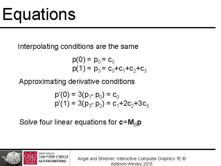
Equations Interpolating conditions are the same p(0) = p 0 = c 0 p(1) = p 3 = c 0+c 1+c 2+c 3 Approximating derivative conditions p’(0) = 3(p 1 - p 0) = c 0 p’(1) = 3(p 3 - p 2) = c 1+2 c 2+3 c 3 Solve four linear equations for c=MBp 41 Angel and Shreiner: Interactive Computer Graphics 7 E © Addison-Wesley 2015

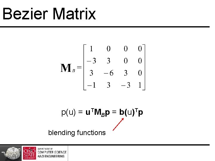
Bezier Matrix p(u) = u. TMBp = b(u)Tp blending functions 42

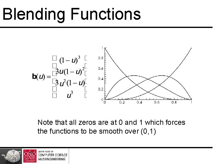
Blending Functions Note that all zeros are at 0 and 1 which forces the functions to be smooth over (0, 1) 43

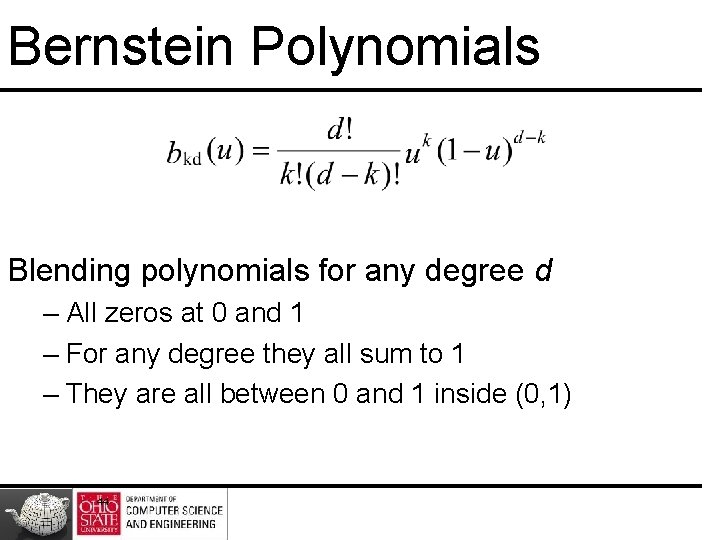
Bernstein Polynomials Blending polynomials for any degree d – All zeros at 0 and 1 – For any degree they all sum to 1 – They are all between 0 and 1 inside (0, 1) 44

Rendering Curves and Surfaces 45

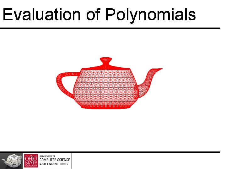
Evaluation of Polynomials 46

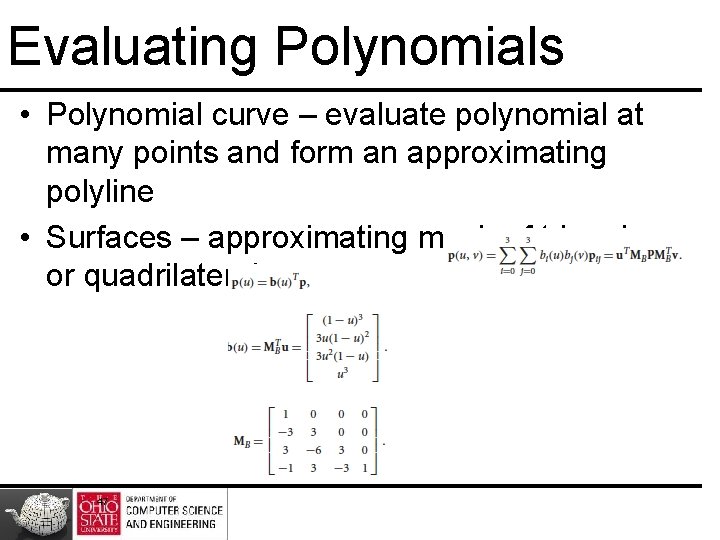
Evaluating Polynomials • Polynomial curve – evaluate polynomial at many points and form an approximating polyline • Surfaces – approximating mesh of triangles or quadrilaterals 47

Evaluate without Computation?

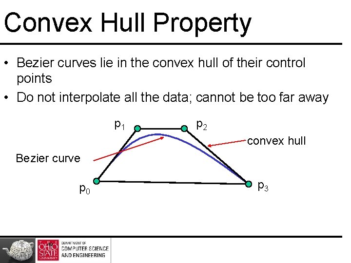
Convex Hull Property • Bezier curves lie in the convex hull of their control points • Do not interpolate all the data; cannot be too far away p 1 p 2 convex hull Bezier curve p 0 49 p 3

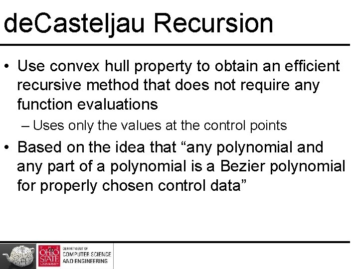
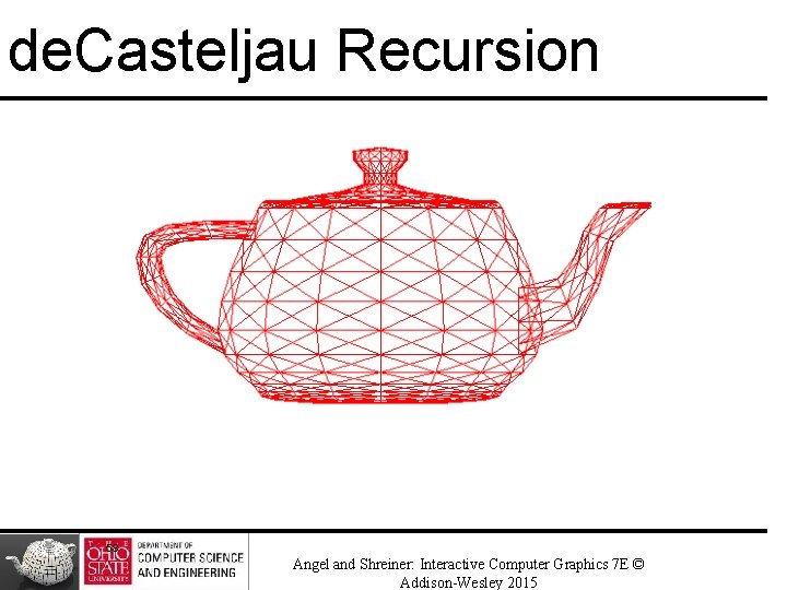
de. Casteljau Recursion • Use convex hull property to obtain an efficient recursive method that does not require any function evaluations – Uses only the values at the control points • Based on the idea that “any polynomial and any part of a polynomial is a Bezier polynomial for properly chosen control data” 50

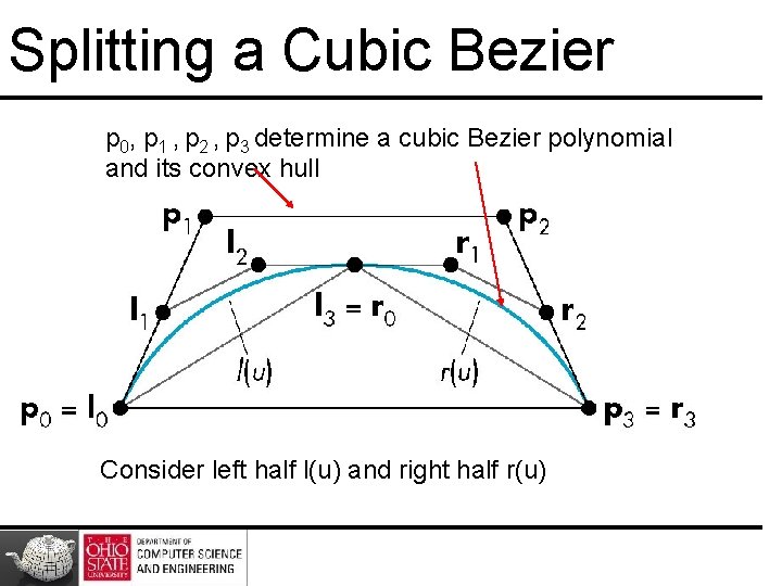
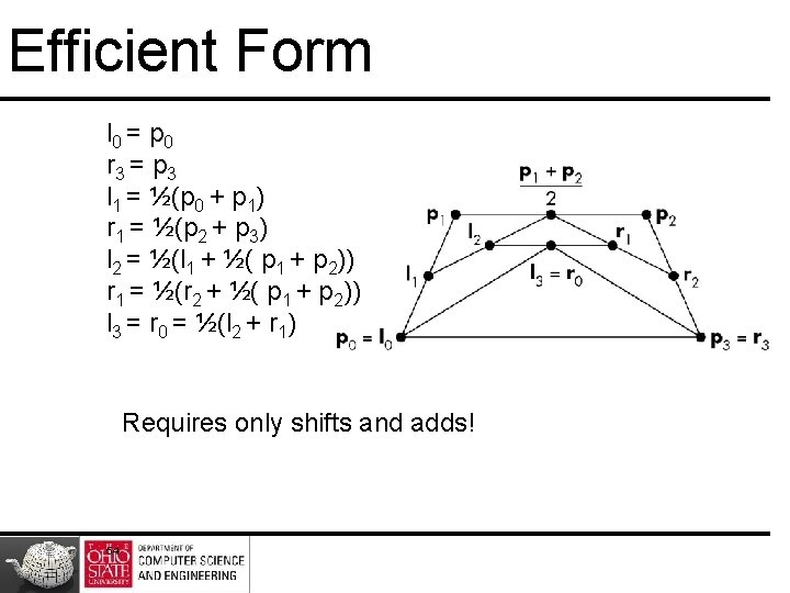
Splitting a Cubic Bezier p 0, p 1 , p 2 , p 3 determine a cubic Bezier polynomial and its convex hull Consider left half l(u) and right half r(u)

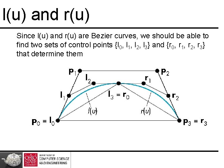
l(u) and r(u) Since l(u) and r(u) are Bezier curves, we should be able to find two sets of control points {l 0, l 1, l 2, l 3} and {r 0, r 1, r 2, r 3} that determine them

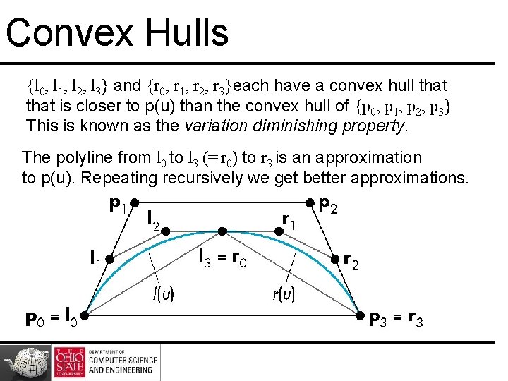
Convex Hulls {l 0, l 1, l 2, l 3} and {r 0, r 1, r 2, r 3}each have a convex hull that is closer to p(u) than the convex hull of {p 0, p 1, p 2, p 3} This is known as the variation diminishing property. The polyline from l 0 to l 3 (= r 0) to r 3 is an approximation to p(u). Repeating recursively we get better approximations.

Efficient Form l 0 = p 0 r 3 = p 3 l 1 = ½(p 0 + p 1) r 1 = ½(p 2 + p 3) l 2 = ½(l 1 + ½( p 1 + p 2)) r 1 = ½(r 2 + ½( p 1 + p 2)) l 3 = r 0 = ½(l 2 + r 1) Requires only shifts and adds! 54

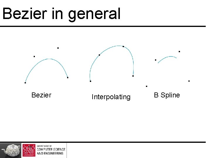
Bezier in general Bezier 55 Interpolating B Spline

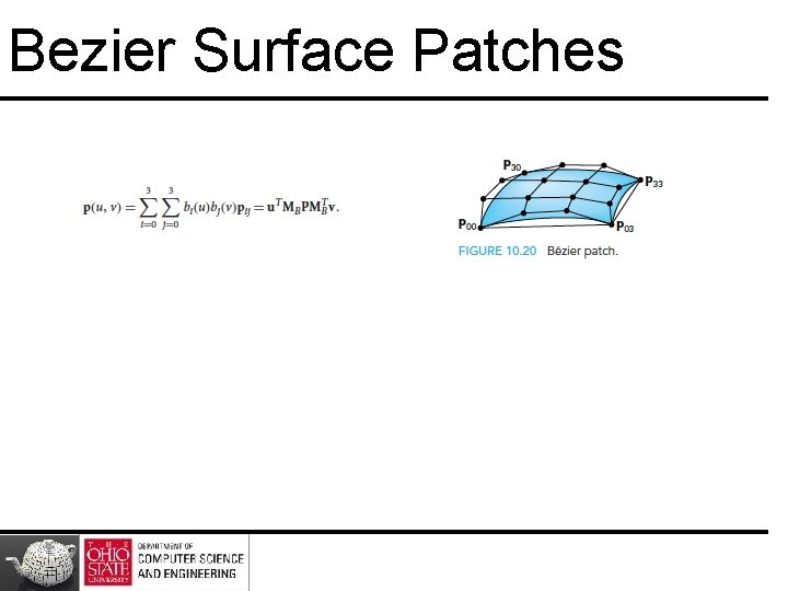
Bezier Patches Using same data array P=[pij] as with interpolating form Patch lies in convex hull

Evaluation of Polynomials 57

de. Casteljau Recursion 58 Angel and Shreiner: Interactive Computer Graphics 7 E © Addison-Wesley 2015

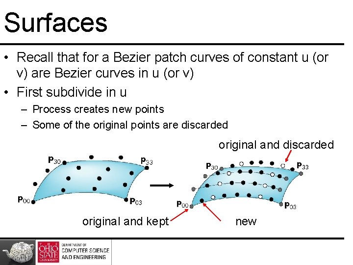
Surfaces • Recall that for a Bezier patch curves of constant u (or v) are Bezier curves in u (or v) • First subdivide in u – Process creates new points – Some of the original points are discarded original and kept new

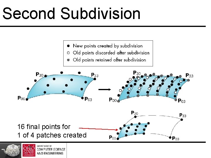
Second Subdivision 16 final points for 1 of 4 patches created 60

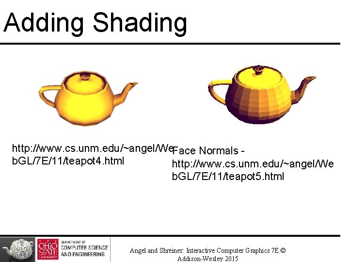
Angel’s Gifts – Chapter 11, 7 e http: //www. cs. unm. edu/~angel/Web. GL/7 E/11/ vertices. js: three versions of the data vertex data patches. js: teapot patch data teapot 1: wire frame teapot by recursive subdivision of Bezier curves teapot 2: wire frame teapot using polynomial evaluation teapot 3: same as teapot 2 with rotation teapot 4: shaded teapot using polynomial evaluation and exact normals teapot 5: shaded teapot using polynomial evaluation and normals computed for each triangle

vertices. js http: //www. cs. unm. edu/~angel/Web. GL/7 E/11/vertices. js var num. Teapot. Vertices = 306; var vertices = [ vec 3(1. 4 , 0. 0 , 2. 4), vec 3(1. 4 , -0. 784 , 2. 4), vec 3(0. 784 , -1. 4 , 2. 4), vec 3(0. 0 , -1. 4 , 2. 4), vec 3(1. 3375 , 0. 0 , 2. 53125), . . . ]; 62

patches. js http: //www. cs. unm. edu/~angel/Web. GL/7 E/11/patches. js var num. Teapot. Patches = 32; var indices = new Array(num. Teapot. Patches); indices[0] = [0, 1, 2, 3, 4, 5, 6, 7, 8, 9, 10, 11, 12, 13, 14, 15 ]; indices[1] = [3, 16, 17, 18, . . ];

Patch Reader http: //www. cs. unm. edu/~angel/Web. GL/7 E/11/pat ch. Reader. js

Bezier Function – Teapot 2 bezier = function(u) { var b = []; var a = 1 -u; b. push(u*u*u); b. push(3*a*a*u); b. push(a*a*a); return b; } 65

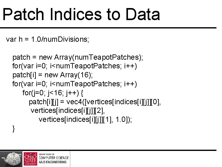
Patch Indices to Data var h = 1. 0/num. Divisions; patch = new Array(num. Teapot. Patches); for(var i=0; i<num. Teapot. Patches; i++) patch[i] = new Array(16); for(var i=0; i<num. Teapot. Patches; i++) for(j=0; j<16; j++) { patch[i][j] = vec 4([vertices[indices[i][j]][0], vertices[indices[i][j]][2], vertices[indices[i][j]][1], 1. 0]); } 66

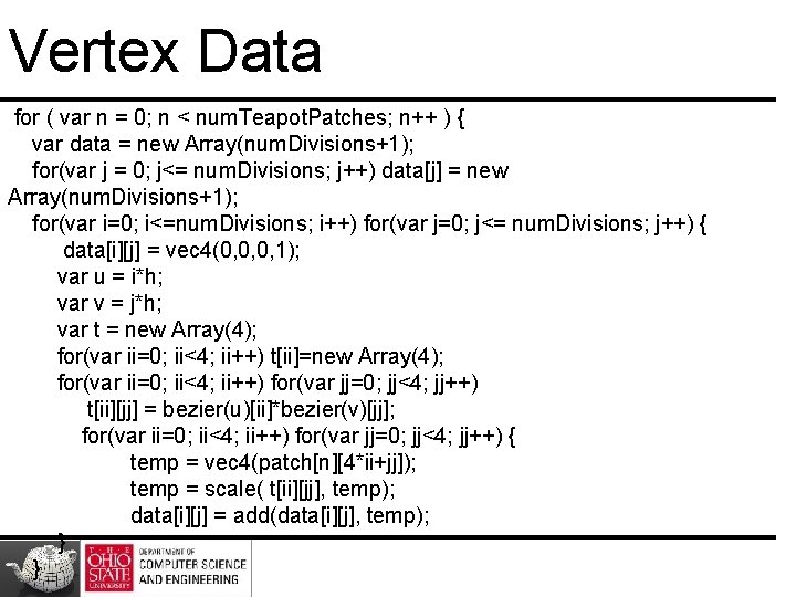
Vertex Data for ( var n = 0; n < num. Teapot. Patches; n++ ) { var data = new Array(num. Divisions+1); for(var j = 0; j<= num. Divisions; j++) data[j] = new Array(num. Divisions+1); for(var i=0; i<=num. Divisions; i++) for(var j=0; j<= num. Divisions; j++) { data[i][j] = vec 4(0, 0, 0, 1); var u = i*h; var v = j*h; var t = new Array(4); for(var ii=0; ii<4; ii++) t[ii]=new Array(4); for(var ii=0; ii<4; ii++) for(var jj=0; jj<4; jj++) t[ii][jj] = bezier(u)[ii]*bezier(v)[jj]; for(var ii=0; ii<4; ii++) for(var jj=0; jj<4; jj++) { temp = vec 4(patch[n][4*ii+jj]); temp = scale( t[ii][jj], temp); data[i][j] = add(data[i][j], temp); } }

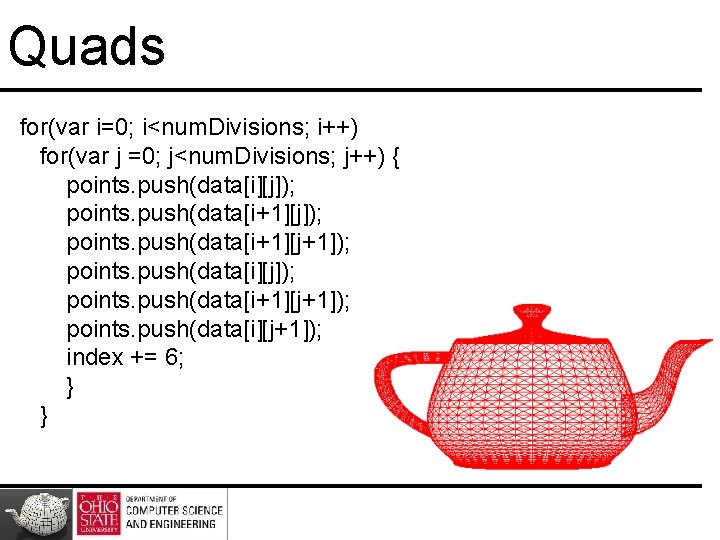
Quads for(var i=0; i<num. Divisions; i++) for(var j =0; j<num. Divisions; j++) { points. push(data[i][j]); points. push(data[i+1][j+1]); points. push(data[i][j+1]); index += 6; } }

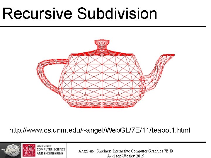
Recursive Subdivision http: //www. cs. unm. edu/~angel/Web. GL/7 E/11/teapot 1. html 69 Angel and Shreiner: Interactive Computer Graphics 7 E © Addison-Wesley 2015

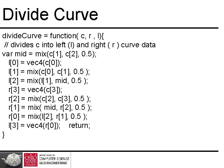
Divide Curve divide. Curve = function( c, r , l){ // divides c into left (l) and right ( r ) curve data var mid = mix(c[1], c[2], 0. 5); l[0] = vec 4(c[0]); l[1] = mix(c[0], c[1], 0. 5 ); l[2] = mix(l[1], mid, 0. 5 ); r[3] = vec 4(c[3]); r[2] = mix(c[2], c[3], 0. 5 ); r[1] = mix( mid, r[2], 0. 5 ); r[0] = mix(l[2], r[1], 0. 5 ); l[3] = vec 4(r[0]); return; }

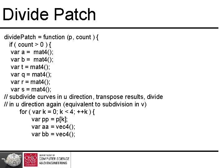
Divide Patch divide. Patch = function (p, count ) { if ( count > 0 ) { var a = mat 4(); var b = mat 4(); var t = mat 4(); var q = mat 4(); var r = mat 4(); var s = mat 4(); // subdivide curves in u direction, transpose results, divide // in u direction again (equivalent to subdivision in v) for ( var k = 0; k < 4; ++k ) { var pp = p[k]; var aa = vec 4(); var bb = vec 4(); 71

Divide Patch divide. Curve( pp, aa, bb ); a[k] = vec 4(aa); b[k] = vec 4(bb); } a = transpose( a ); b = transpose( b ); for ( var k = 0; k < 4; ++k ) { var pp = vec 4(a[k]); var aa = vec 4(); var bb = vec 4(); divide. Curve( pp, aa, bb ); q[k] = vec 4(aa); r[k] = vec 4(bb); } for ( var k = 0; k < 4; ++k ) { var pp = vec 4(b[k]); var aa = vec 4(); 72

Divide Patch var bb = vec 4(); divide. Curve( pp, aa, bb ); t[k] = vec 4(bb); } // recursive division of 4 resulting patches divide. Patch( q, count - 1 ); divide. Patch( r, count - 1 ); divide. Patch( s, count - 1 ); divide. Patch( t, count - 1 ); } else { draw. Patch( p ); } return; } 73

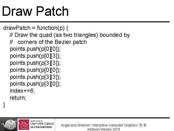
Draw Patch draw. Patch = function(p) { // Draw the quad (as two triangles) bounded by // corners of the Bezier patch points. push(p[0][0]); points. push(p[0][3]); points. push(p[3][3]); points. push(p[0][0]); points. push(p[3][3]); points. push(p[3][0]); index+=6; return; } 74 Angel and Shreiner: Interactive Computer Graphics 7 E © Addison-Wesley 2015

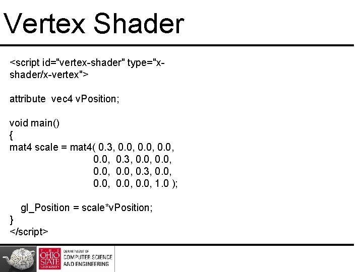
Vertex Shader <script id="vertex-shader" type="xshader/x-vertex"> attribute vec 4 v. Position; void main() { mat 4 scale = mat 4( 0. 3, 0. 0, 0. 0, 1. 0 ); gl_Position = scale*v. Position; } </script>

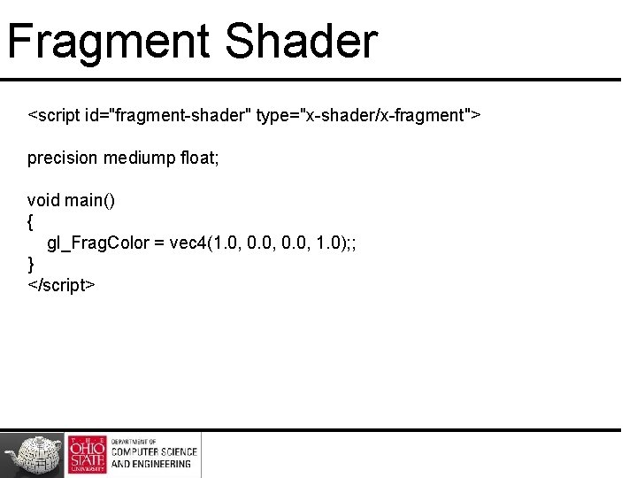
Fragment Shader <script id="fragment-shader" type="x-shader/x-fragment"> precision mediump float; void main() { gl_Frag. Color = vec 4(1. 0, 0. 0, 1. 0); ; } </script>

Adding Shading http: //www. cs. unm. edu/~angel/We. Face Normals b. GL/7 E/11/teapot 4. html http: //www. cs. unm. edu/~angel/We b. GL/7 E/11/teapot 5. html 77 Angel and Shreiner: Interactive Computer Graphics 7 E © Addison-Wesley 2015

Using Face Normals var t 1 = subtract(data[i+1][j], data[i][j]); var t 2 =subtract(data[i+1][j+1], data[i][j]); var normal = cross(t 1, t 2); normal = normalize(normal); normal[3] = 0; points. push(data[i][j]); normals. push(normal); points. push(data[i+1][j+1]); normals. push(normal); points. push(data[i][j+1]); normals. push(normal); index+= 6; 78

Exact Normals nbezier = function(u) { var b = []; b. push(3*u*u); b. push(3*u*(2 -3*u)); b. push(3*(1 -4*u+3*u*u)); b. push(-3*(1 -u)); return b; }

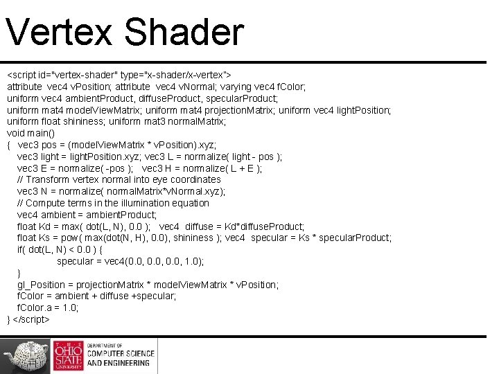
Vertex Shader <script id="vertex-shader" type="x-shader/x-vertex”> attribute vec 4 v. Position; attribute vec 4 v. Normal; varying vec 4 f. Color; uniform vec 4 ambient. Product, diffuse. Product, specular. Product; uniform mat 4 model. View. Matrix; uniform mat 4 projection. Matrix; uniform vec 4 light. Position; uniform float shininess; uniform mat 3 normal. Matrix; void main() { vec 3 pos = (model. View. Matrix * v. Position). xyz; vec 3 light = light. Position. xyz; vec 3 L = normalize( light - pos ); vec 3 E = normalize( -pos ); vec 3 H = normalize( L + E ); // Transform vertex normal into eye coordinates vec 3 N = normalize( normal. Matrix*v. Normal. xyz); // Compute terms in the illumination equation vec 4 ambient = ambient. Product; float Kd = max( dot(L, N), 0. 0 ); vec 4 diffuse = Kd*diffuse. Product; float Ks = pow( max(dot(N, H), 0. 0), shininess ); vec 4 specular = Ks * specular. Product; if( dot(L, N) < 0. 0 ) { specular = vec 4(0. 0, 1. 0); } gl_Position = projection. Matrix * model. View. Matrix * v. Position; f. Color = ambient + diffuse +specular; f. Color. a = 1. 0; } </script>

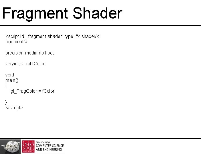
Fragment Shader <script id="fragment-shader" type="x-shader/xfragment"> precision mediump float; varying vec 4 f. Color; void main() { gl_Frag. Color = f. Color; } </script>

Post Geometry Shaders

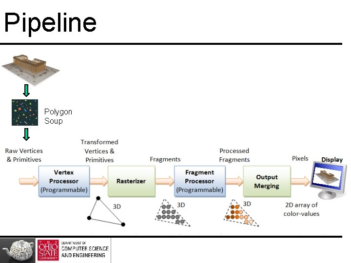
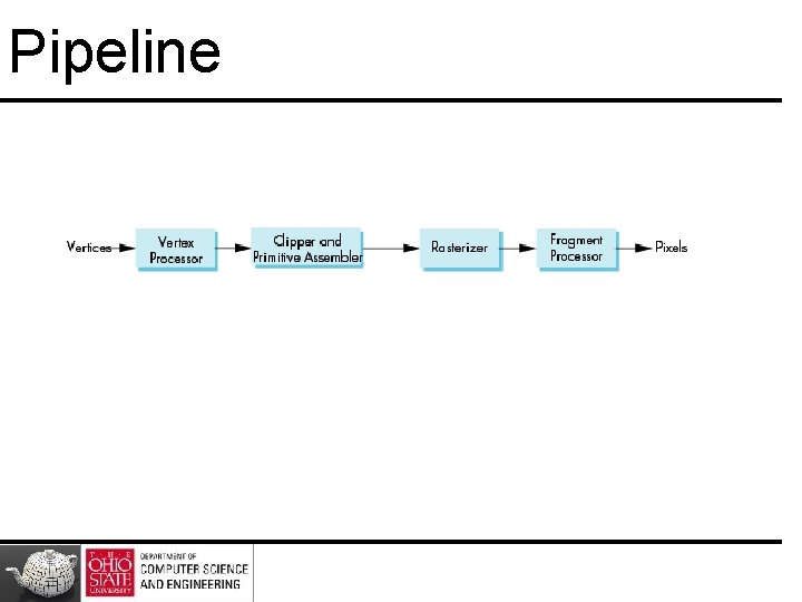
Pipeline Polygon Soup

Pipeline

Topics • Clipping • Scan conversion

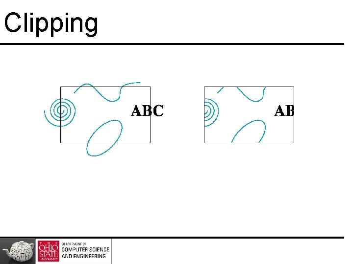
Clipping

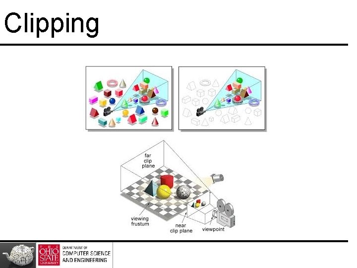
Clipping • After geometric stage – vertices assembled into primitives • Must clip primitives that are outside view frustum

Clipping

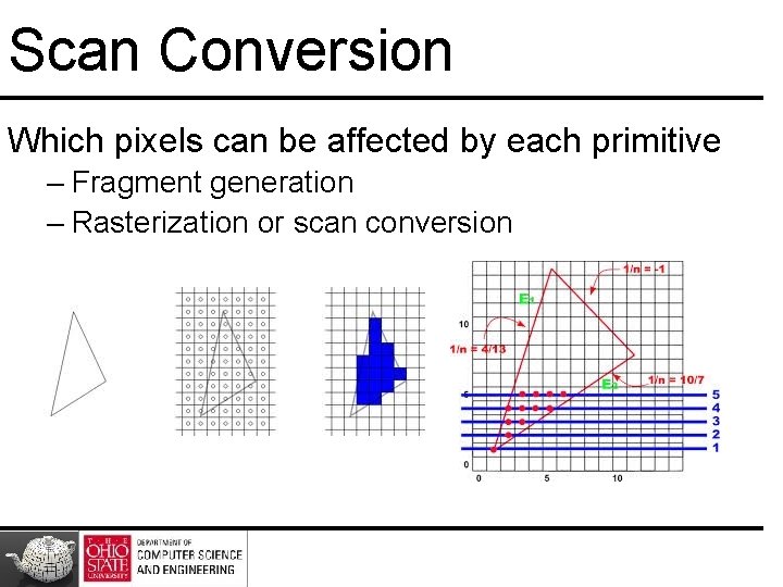
Scan Conversion Which pixels can be affected by each primitive – Fragment generation – Rasterization or scan conversion

Additional Tasks Some tasks deferred until fragment processing – Hidden surface removal – Antialiasing

Clipping

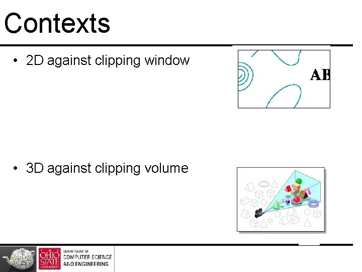
Contexts • 2 D against clipping window • 3 D against clipping volume

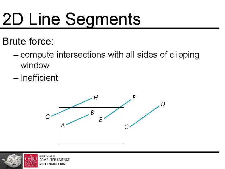
2 D Line Segments Brute force: – compute intersections with all sides of clipping window – Inefficient

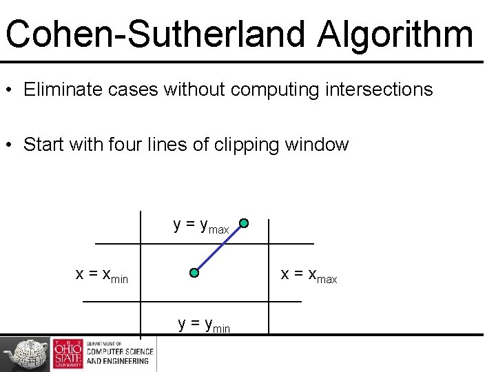
Cohen-Sutherland Algorithm • Eliminate cases without computing intersections • Start with four lines of clipping window y = ymax x = xmin x = xmax y = ymin

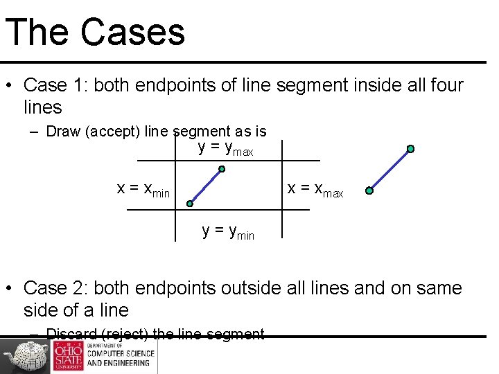
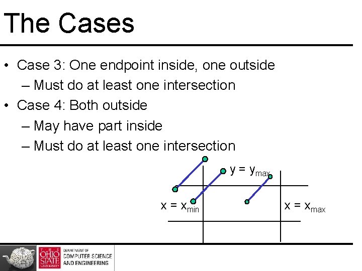
The Cases • Case 1: both endpoints of line segment inside all four lines – Draw (accept) line segment as is y = ymax x = xmin x = xmax y = ymin • Case 2: both endpoints outside all lines and on same side of a line – Discard (reject) the line segment

The Cases • Case 3: One endpoint inside, one outside – Must do at least one intersection • Case 4: Both outside – May have part inside – Must do at least one intersection y = ymax x = xmin x = xmax

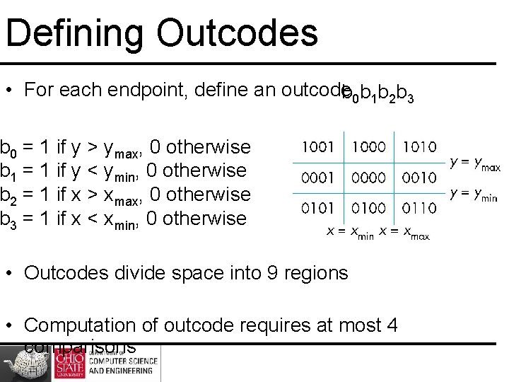
Defining Outcodes • For each endpoint, define an outcode b 0 b 1 b 2 b 3 b 0 = 1 if y > ymax, 0 otherwise b 1 = 1 if y < ymin, 0 otherwise b 2 = 1 if x > xmax, 0 otherwise b 3 = 1 if x < xmin, 0 otherwise • Outcodes divide space into 9 regions • Computation of outcode requires at most 4 comparisons

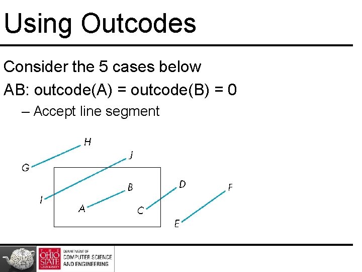
Using Outcodes Consider the 5 cases below AB: outcode(A) = outcode(B) = 0 – Accept line segment

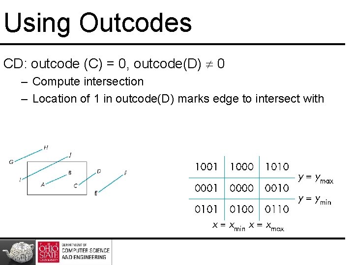
Using Outcodes CD: outcode (C) = 0, outcode(D) 0 – Compute intersection – Location of 1 in outcode(D) marks edge to intersect with

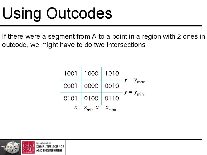
Using Outcodes If there were a segment from A to a point in a region with 2 ones in outcode, we might have to do two intersections

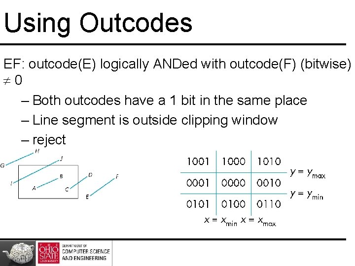
Using Outcodes EF: outcode(E) logically ANDed with outcode(F) (bitwise) 0 – Both outcodes have a 1 bit in the same place – Line segment is outside clipping window – reject

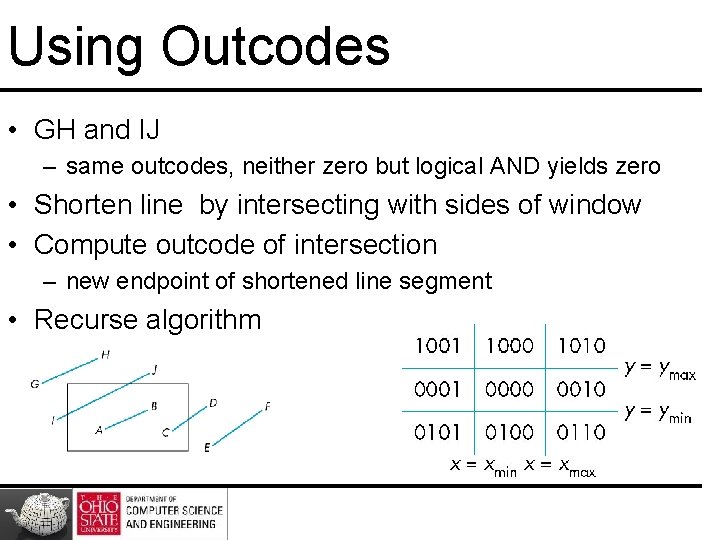
Using Outcodes • GH and IJ – same outcodes, neither zero but logical AND yields zero • Shorten line by intersecting with sides of window • Compute outcode of intersection – new endpoint of shortened line segment • Recurse algorithm

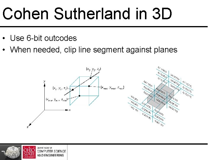
Cohen Sutherland in 3 D • Use 6 -bit outcodes • When needed, clip line segment against planes

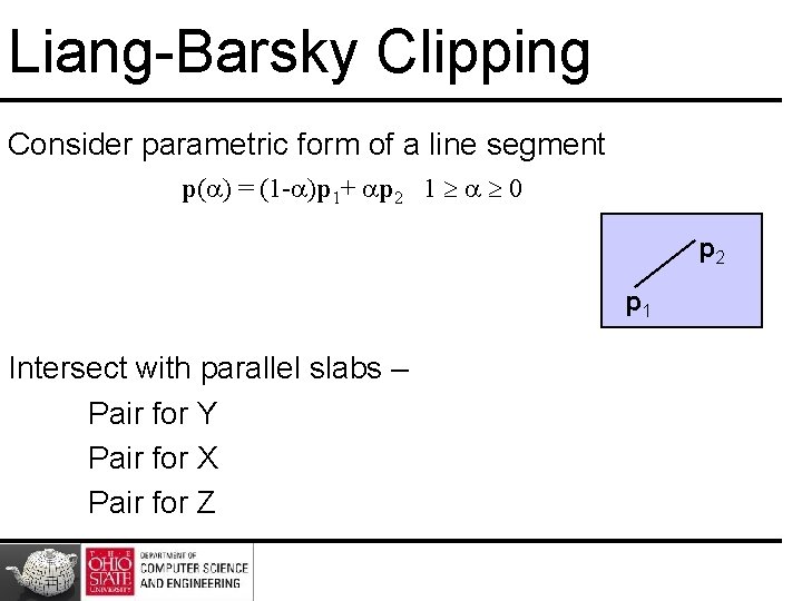
Liang-Barsky Clipping Consider parametric form of a line segment p(a) = (1 -a)p 1+ ap 2 1 a 0 p 2 p 1 Intersect with parallel slabs – Pair for Y Pair for X Pair for Z

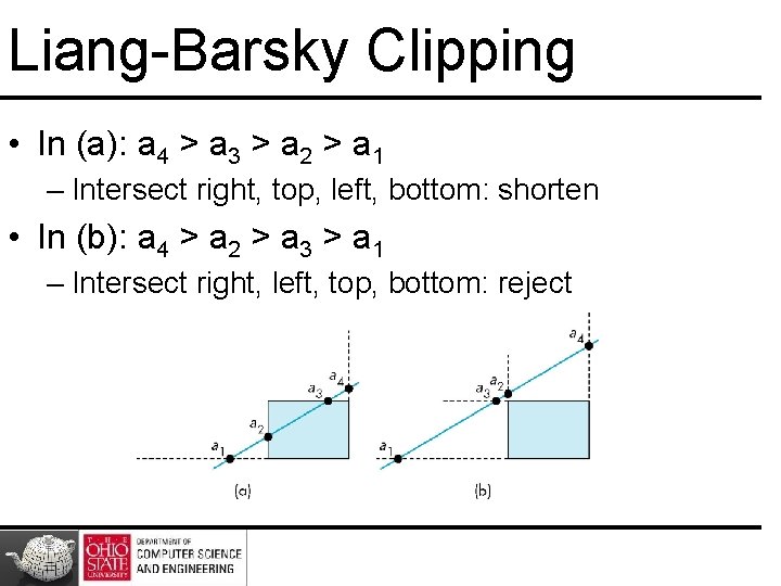
Liang-Barsky Clipping • In (a): a 4 > a 3 > a 2 > a 1 – Intersect right, top, left, bottom: shorten • In (b): a 4 > a 2 > a 3 > a 1 – Intersect right, left, top, bottom: reject

Advantages • Can accept/reject as easily as with Cohen. Sutherland • Using values of a, we do not have to use algorithm recursively as with C-S • Extends to 3 D

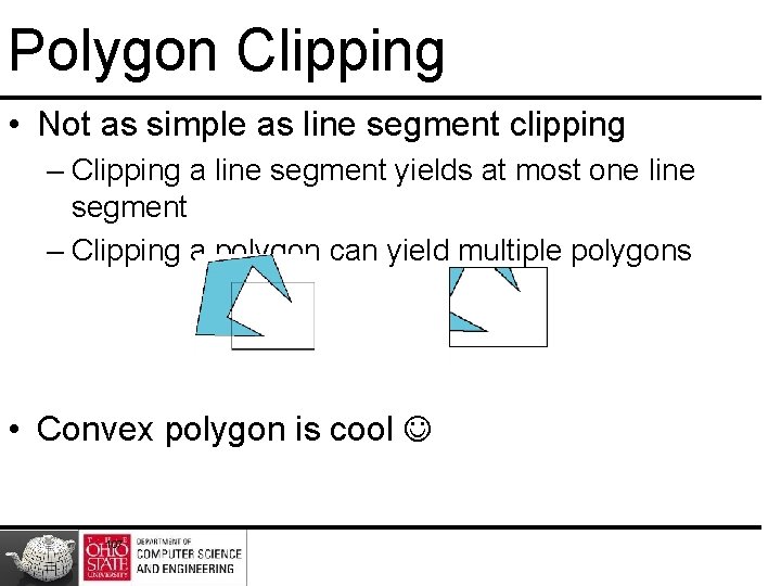
Polygon Clipping • Not as simple as line segment clipping – Clipping a line segment yields at most one line segment – Clipping a polygon can yield multiple polygons • Convex polygon is cool 107

Fixes

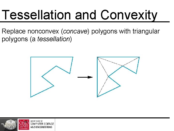
Tessellation and Convexity Replace nonconvex (concave) polygons with triangular polygons (a tessellation) 109

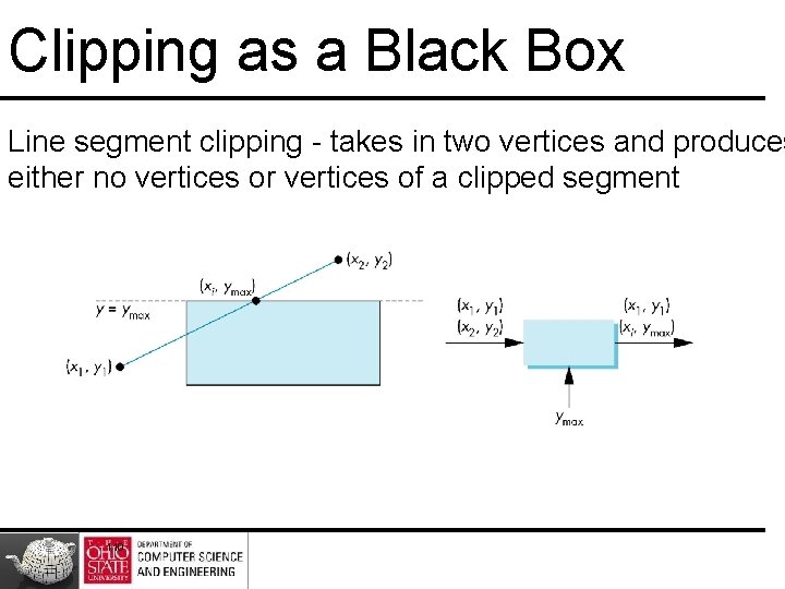
Clipping as a Black Box Line segment clipping - takes in two vertices and produces either no vertices or vertices of a clipped segment 110

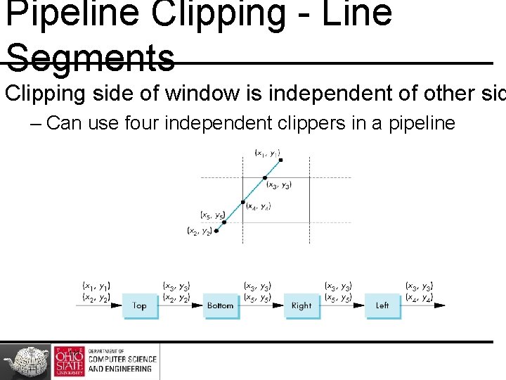
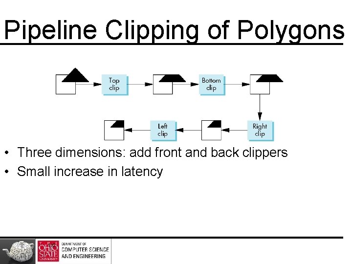
Pipeline Clipping - Line Segments Clipping side of window is independent of other sid – Can use four independent clippers in a pipeline 111

Pipeline Clipping of Polygons • Three dimensions: add front and back clippers • Small increase in latency 112

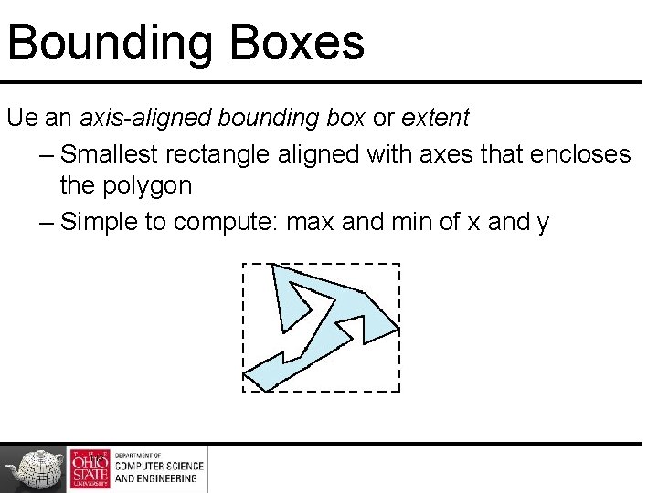
Bounding Boxes Ue an axis-aligned bounding box or extent – Smallest rectangle aligned with axes that encloses the polygon – Simple to compute: max and min of x and y 113

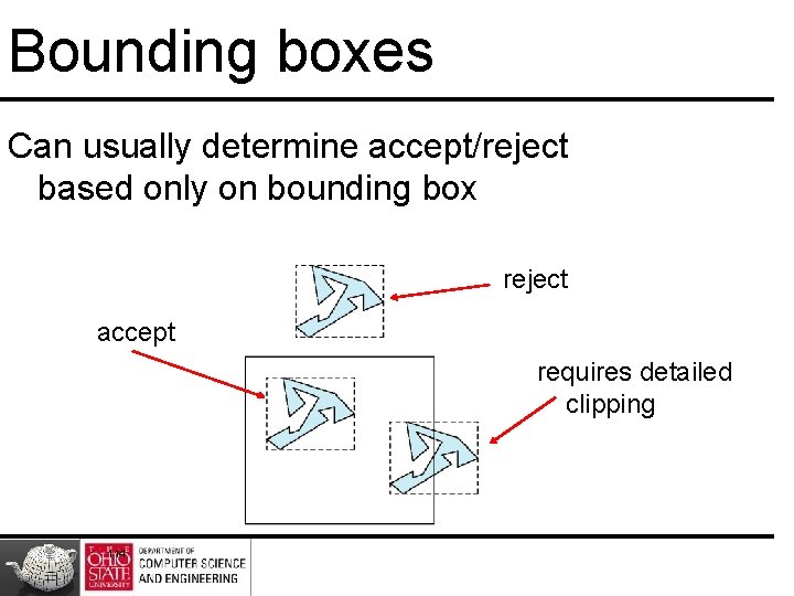
Bounding boxes Can usually determine accept/reject based only on bounding box reject accept requires detailed clipping 114

Clipping vs. Visibility • Clipping similar to hidden-surface removal • Remove objects that are not visible to the camera • Use visibility or occlusion testing early in the process to eliminate as many polygons as possible before going through the entire pipeline 115

Clipping

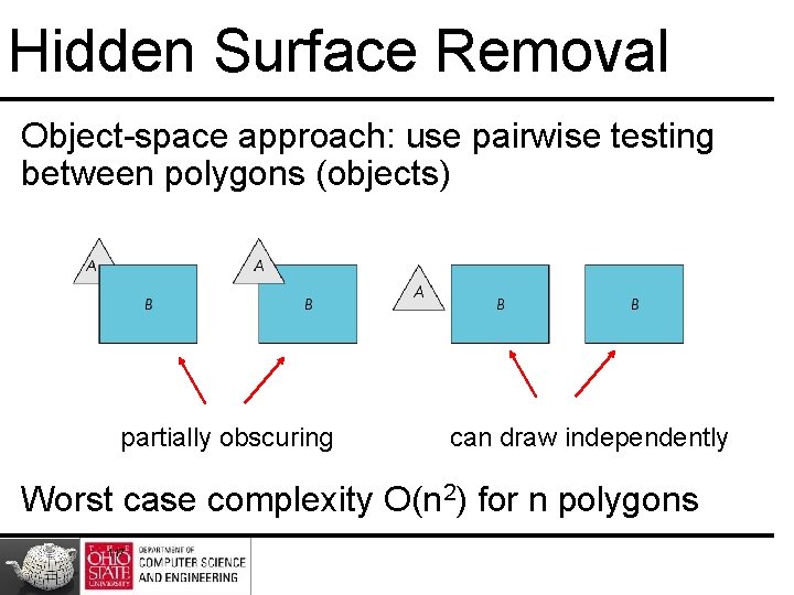
Hidden Surface Removal Object-space approach: use pairwise testing between polygons (objects) partially obscuring can draw independently Worst case complexity O(n 2) for n polygons 117

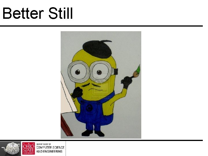
Better Still

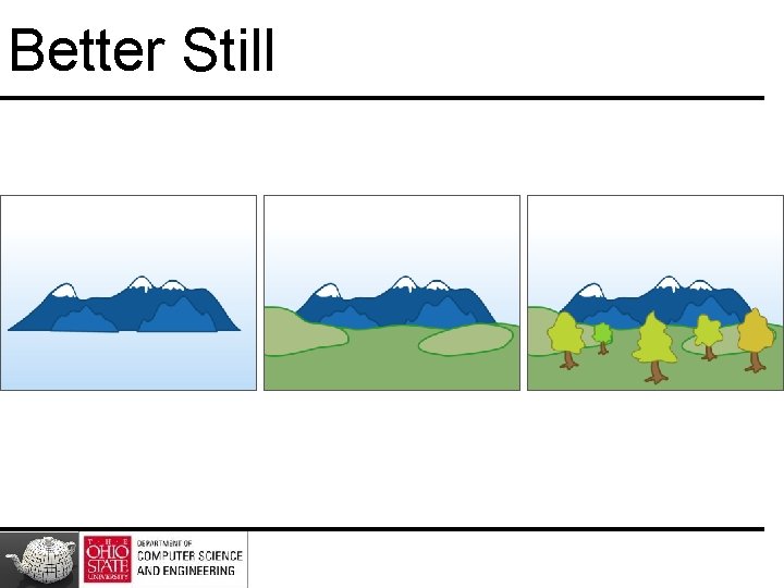
Better Still

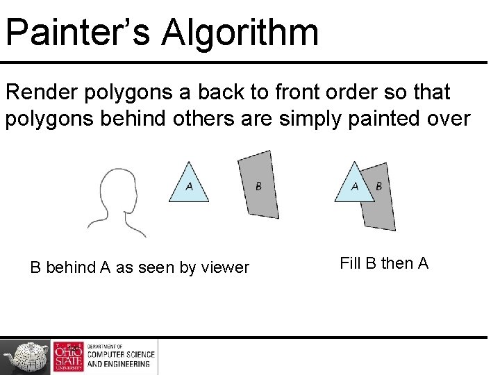
Painter’s Algorithm Render polygons a back to front order so that polygons behind others are simply painted over B behind A as seen by viewer 120 Fill B then A

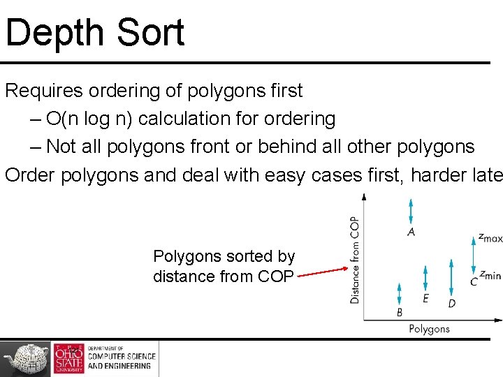
Depth Sort Requires ordering of polygons first – O(n log n) calculation for ordering – Not all polygons front or behind all other polygons Order polygons and deal with easy cases first, harder late Polygons sorted by distance from COP 121

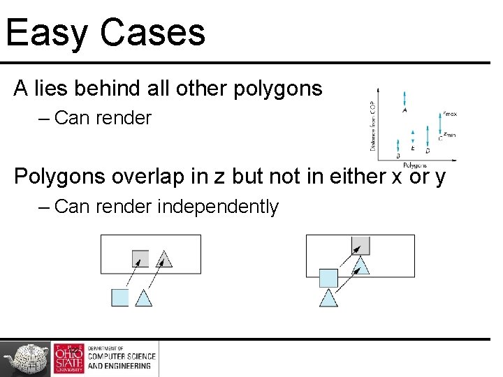
Easy Cases A lies behind all other polygons – Can render Polygons overlap in z but not in either x or y – Can render independently 122

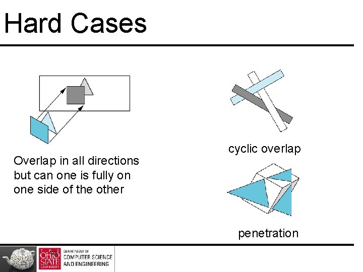
Hard Cases Overlap in all directions but can one is fully on one side of the other cyclic overlap penetration 123

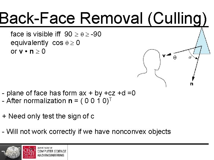
Back-Face Removal (Culling) face is visible iff 90 -90 equivalently cos 0 or v • n 0 - plane of face has form ax + by +cz +d =0 - After normalization n = ( 0 0 1 0)T + Need only test the sign of c - Will not work correctly if we have nonconvex objects 124

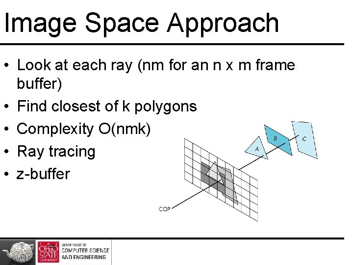
Image Space Approach • Look at each ray (nm for an n x m frame buffer) • Find closest of k polygons • Complexity O(nmk) • Ray tracing • z-buffer 125

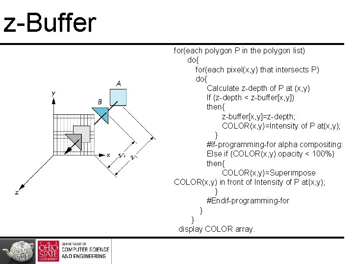
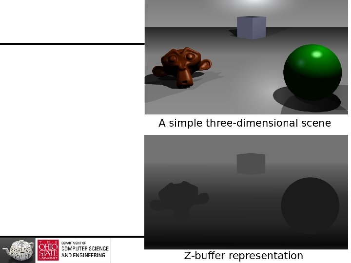
z-Buffer Algorithm • Use a buffer called z or depth buffer to store depth of closest object at each pixel found so far • As we render each polygon, compare the depth of each pixel to depth in z buffer • If less, place shade of pixel in color buffer and update z buffer 126

z-Buffer for(each polygon P in the polygon list) do{ for(each pixel(x, y) that intersects P) do{ Calculate z-depth of P at (x, y) If (z-depth < z-buffer[x, y]) then{ z-buffer[x, y]=z-depth; COLOR(x, y)=Intensity of P at(x, y); } #If-programming-for alpha compositing: Else if (COLOR(x, y). opacity < 100%) then{ COLOR(x, y)=Superimpose COLOR(x, y) in front of Intensity of P at(x, y); } #Endif-programming-for } } display COLOR array.

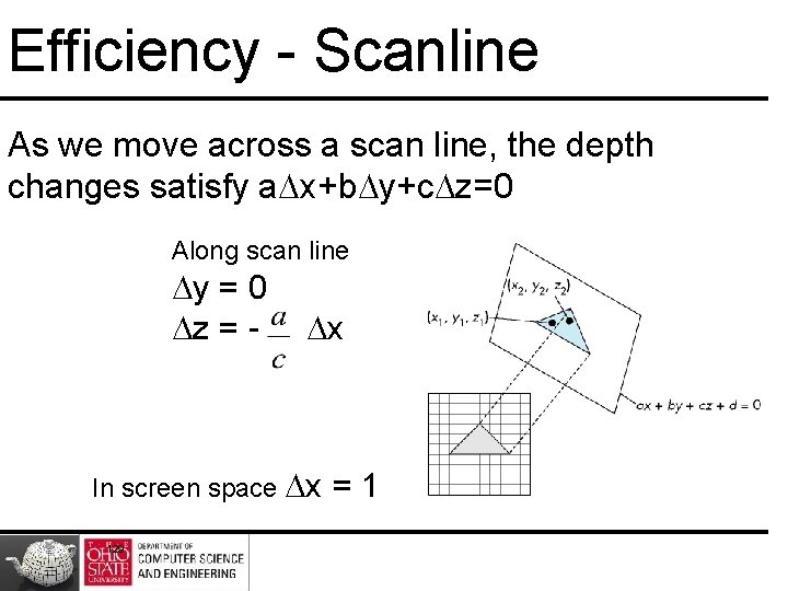
Efficiency - Scanline As we move across a scan line, the depth changes satisfy a x+b y+c z=0 Along scan line y = 0 z = - x In screen space x 129 =1

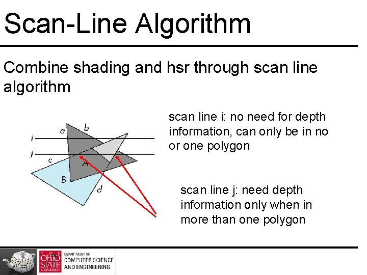
Scan-Line Algorithm Combine shading and hsr through scan line algorithm scan line i: no need for depth information, can only be in no or one polygon scan line j: need depth information only when in more than one polygon 130

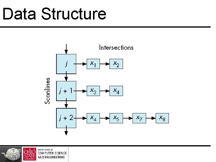
Implementation Need a data structure to store – Flag for each polygon (inside/outside) – Incremental structure for scan lines that stores which edges are encountered – Parameters for planes 131

Rasterization • Rasterization (scan conversion) – Determine which pixels that are inside primitive specified by a set of vertices – Produces a set of fragments – Fragments have a location (pixel location) and other attributes such color and texture coordinates that are determined by interpolating values at vertices • Pixel colors determined later using color, texture, and other vertex properties

Scan-Line Rasterization

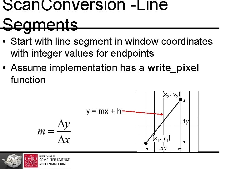
Scan. Conversion -Line Segments • Start with line segment in window coordinates with integer values for endpoints • Assume implementation has a write_pixel function y = mx + h

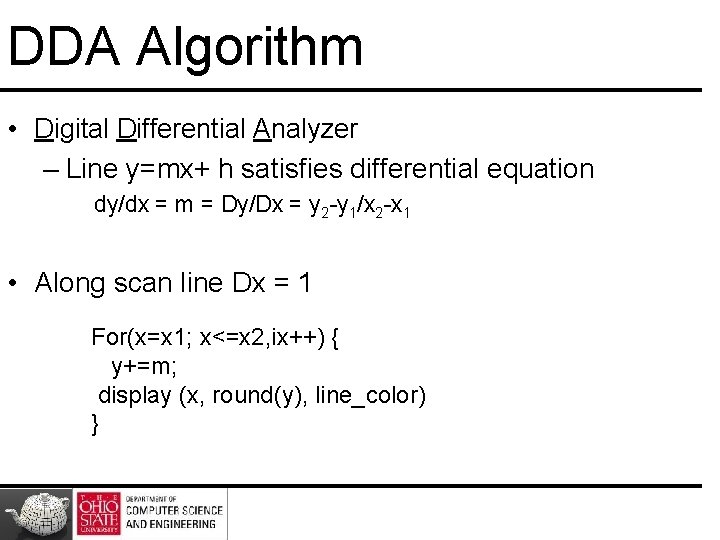
DDA Algorithm • Digital Differential Analyzer – Line y=mx+ h satisfies differential equation dy/dx = m = Dy/Dx = y 2 -y 1/x 2 -x 1 • Along scan line Dx = 1 For(x=x 1; x<=x 2, ix++) { y+=m; display (x, round(y), line_color) }

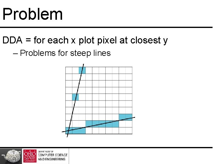
Problem DDA = for each x plot pixel at closest y – Problems for steep lines

Bresenham’s Algorithm • DDA requires one floating point addition per step • Eliminate computations through Bresenham’s algorithm • Consider only 1 m 0 – Other cases by symmetry • Assume pixel centers are at half integers

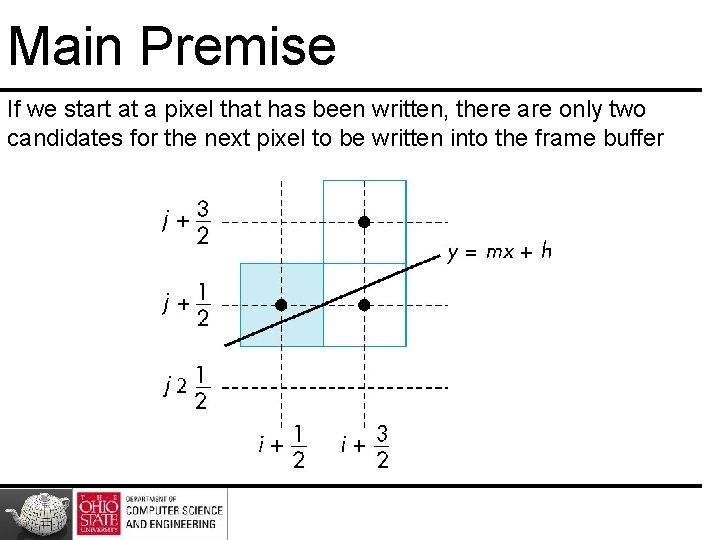
Main Premise If we start at a pixel that has been written, there are only two candidates for the next pixel to be written into the frame buffer

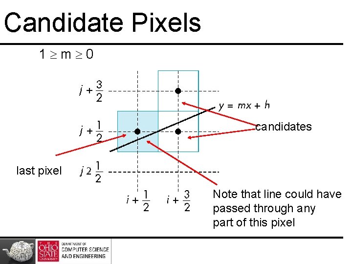
Candidate Pixels 1 m 0 candidates last pixel Note that line could have passed through any part of this pixel

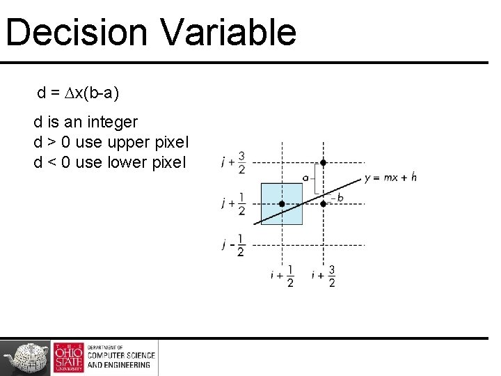
Decision Variable d = x(b-a) d is an integer d > 0 use upper pixel d < 0 use lower pixel -

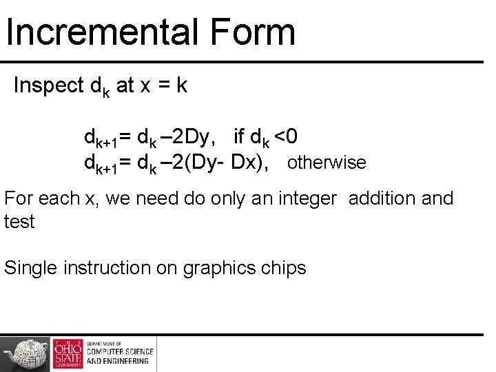
Incremental Form Inspect dk at x = k dk+1= dk – 2 Dy, if dk <0 dk+1= dk – 2(Dy- Dx), otherwise For each x, we need do only an integer addition and test Single instruction on graphics chips

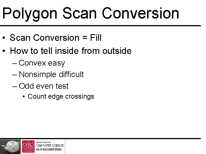
Polygon Scan Conversion • Scan Conversion = Fill • How to tell inside from outside – Convex easy – Nonsimple difficult – Odd even test • Count edge crossings

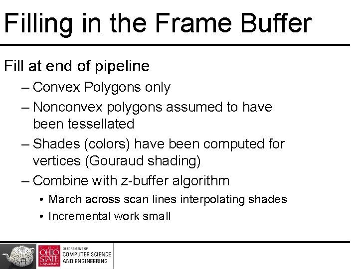
Filling in the Frame Buffer Fill at end of pipeline – Convex Polygons only – Nonconvex polygons assumed to have been tessellated – Shades (colors) have been computed for vertices (Gouraud shading) – Combine with z-buffer algorithm • March across scan lines interpolating shades • Incremental work small

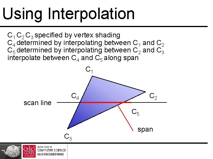
Using Interpolation C 1 C 2 C 3 specified by vertex shading C 4 determined by interpolating between C 1 and C 2 C 5 determined by interpolating between C 2 and C 3 interpolate between C 4 and C 5 along span C 1 scan line C 4 C 2 C 5 C 3 span

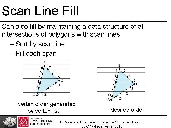
Scan Line Fill Can also fill by maintaining a data structure of all intersections of polygons with scan lines – Sort by scan line – Fill each span vertex order generated by vertex list desired order E. Angel and D. Shreiner: Interactive Computer Graphics 6 E © Addison-Wesley 2012

Data Structure

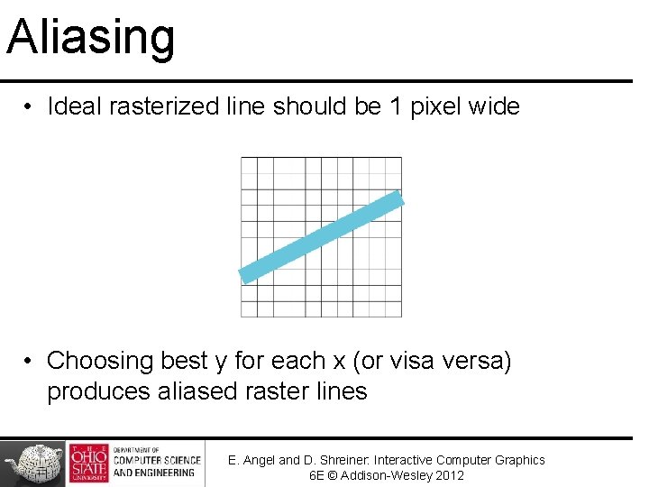
Aliasing • Ideal rasterized line should be 1 pixel wide • Choosing best y for each x (or visa versa) produces aliased raster lines E. Angel and D. Shreiner: Interactive Computer Graphics 6 E © Addison-Wesley 2012

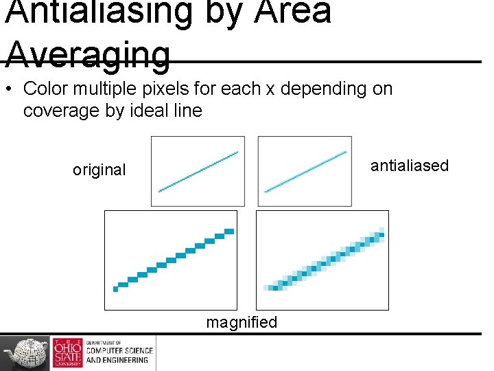
Antialiasing by Area Averaging • Color multiple pixels for each x depending on coverage by ideal line antialiased original magnified

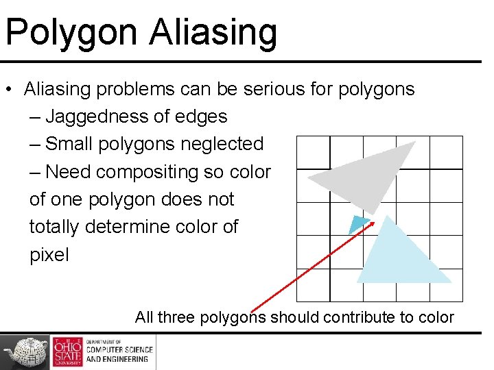
Polygon Aliasing • Aliasing problems can be serious for polygons – Jaggedness of edges – Small polygons neglected – Need compositing so color of one polygon does not totally determine color of pixel All three polygons should contribute to color