Direct Volume Rendering DVR Raycasting Jian Huang This

Direct Volume Rendering (DVR): Ray-casting Jian Huang This set of slides references slides used by Prof. Torsten Moeller (Simon Fraser), Prof. Han-Wei Shen (Ohio State).

Papers • Tuy and Tuy, 1984, IEEE CG & A (one of the earliest volume rendering techniques) • Levoy, 1988 IEEE CG&A, and later improvements • Drebin, Carpenter, Hanrahan, 1988, SIGGRAPH Direct: No conversion to surface geometry

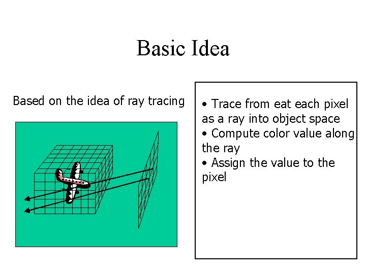
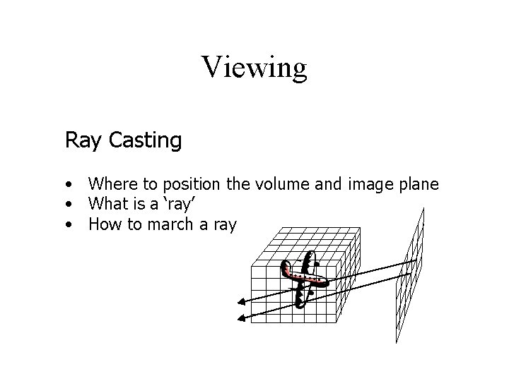
Basic Idea Based on the idea of ray tracing • Trace from eat each pixel as a ray into object space • Compute color value along the ray • Assign the value to the pixel

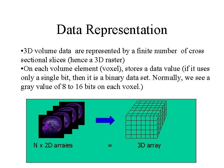
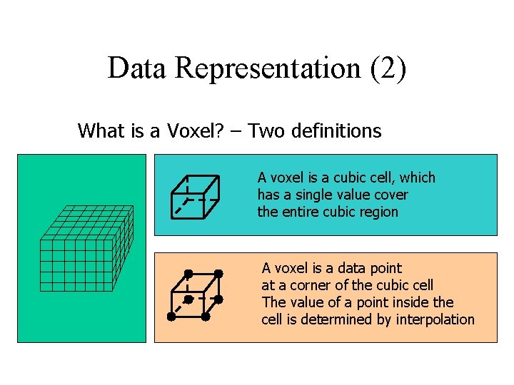
Data Representation • 3 D volume data are represented by a finite number of cross sectional slices (hence a 3 D raster) • On each volume element (voxel), stores a data value (if it uses only a single bit, then it is a binary data set. Normally, we see a gray value of 8 to 16 bits on each voxel. ) N x 2 D arraies = 3 D array

Data Representation (2) What is a Voxel? – Two definitions A voxel is a cubic cell, which has a single value cover the entire cubic region A voxel is a data point at a corner of the cubic cell The value of a point inside the cell is determined by interpolation

Viewing Ray Casting • Where to position the volume and image plane • What is a ‘ray’ • How to march a ray

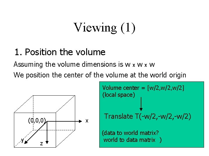
Viewing (1) 1. Position the volume Assuming the volume dimensions is w x wxw We position the center of the volume at the world origin Volume center = [w/2, w/2] (local space) (0, 0, 0) y z x Translate T(-w/2, -w/2) (data to world matrix? world to data matrix )

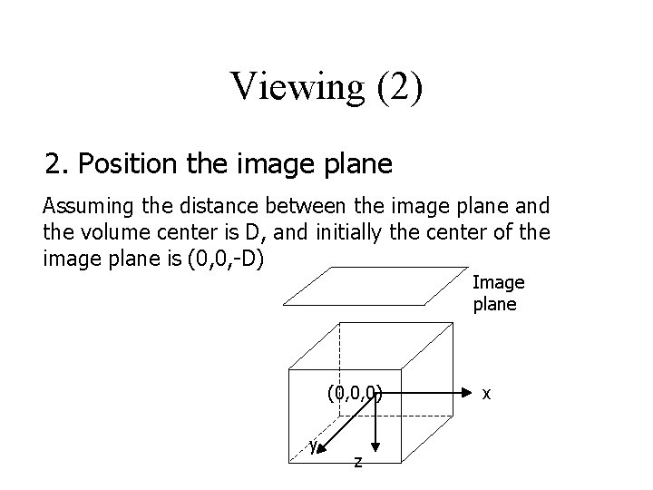
Viewing (2) 2. Position the image plane Assuming the distance between the image plane and the volume center is D, and initially the center of the image plane is (0, 0, -D) Image plane (0, 0, 0) y z x

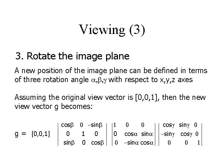
Viewing (3) 3. Rotate the image plane A new position of the image plane can be defined in terms of three rotation angle , b, g with respect to x, y, z axes Assuming the original view vector is [0, 0, 1], then the new view vector g becomes: g = [0, 0, 1] cosb 0 -sinb 0 1 0 sinb 0 cosb 1 0 0 cos sin -sin cosg sing 0 -sing cosg 0 0 0 1

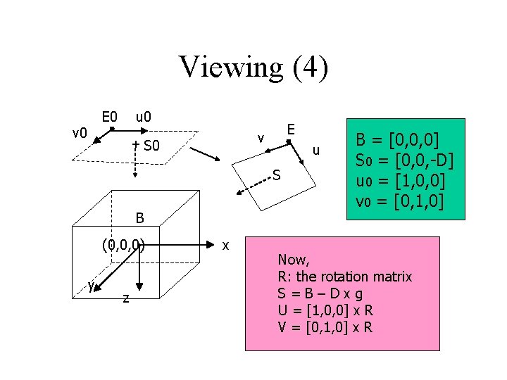
Viewing (4) E 0 v 0 u 0 E v + S 0 u S B (0, 0, 0) y z x B = [0, 0, 0] S 0 = [0, 0, -D] u 0 = [1, 0, 0] v 0 = [0, 1, 0] Now, R: the rotation matrix S=B–Dxg U = [1, 0, 0] x R V = [0, 1, 0] x R

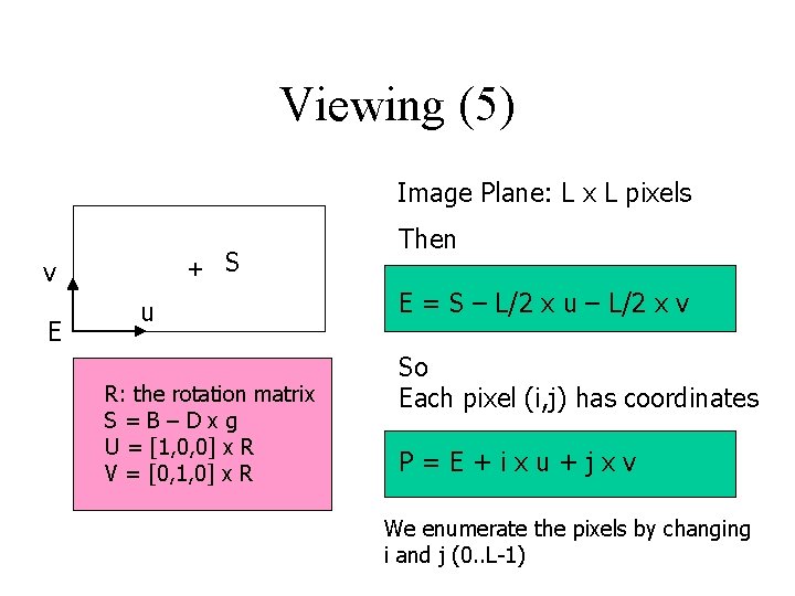
Viewing (5) Image Plane: L x L pixels + v E S u R: the rotation matrix S=B–Dxg U = [1, 0, 0] x R V = [0, 1, 0] x R Then E = S – L/2 x u – L/2 x v So Each pixel (i, j) has coordinates P=E+ixu+jxv We enumerate the pixels by changing i and j (0. . L-1)

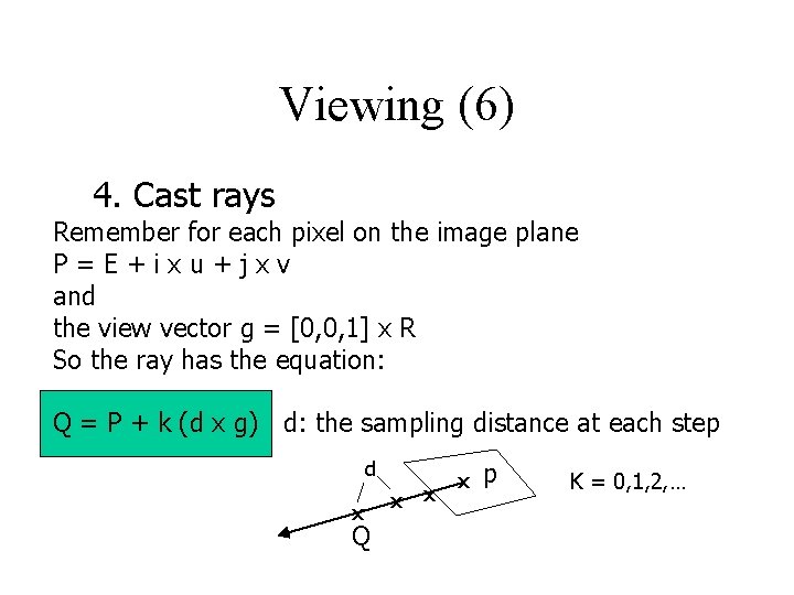
Viewing (6) 4. Cast rays Remember for each pixel on the image plane P=E+ixu+jxv and the view vector g = [0, 0, 1] x R So the ray has the equation: Q = P + k (d x g) d: the sampling distance at each step d x Q x x x p K = 0, 1, 2, …

Early Methods • Before 1988 • Did not consider transparency • did not consider sophisticated light transportation theory • were concerned with quick solutions • hence more or less applied to binary data non-binary data require sophisticated classification/compositing methods!

Ray Tracing -> Ray Casting • “another” typical method from traditional graphics • Typically we only deal with primary rays hence: ray-casting • a natural image-order technique • as opposed to surface graphics - how do we calculate the ray/surface intersection? ? ? • Since we have no surfaces - we need to carefully step through the volume

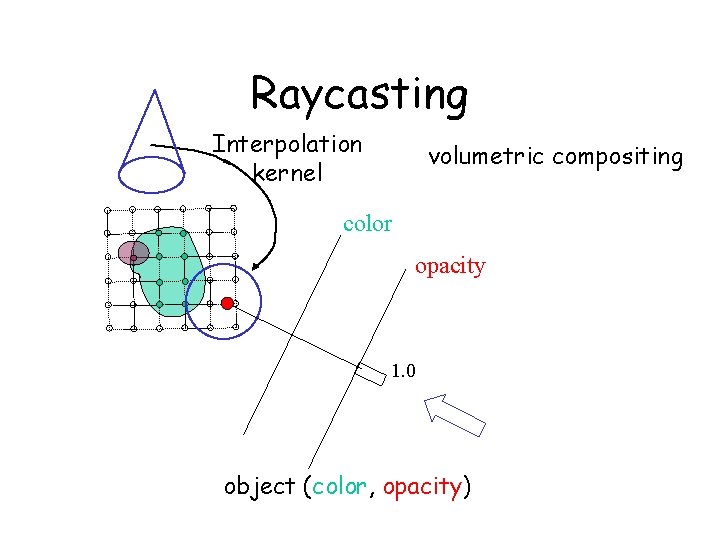
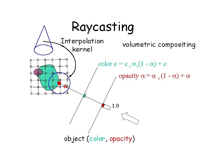
Ray Casting • Stepping through the volume: a ray is cast into the volume, sampling the volume at certain intervals • The sampling intervals are usually equi-distant, but don’t have to be (e. g. importance sampling) • At each sampling location, a sample is interpolated / reconstructed from the grid voxels • popular filters are: nearest neighbor (box), trilinear (tent), Gaussian, cubic spline • Along the ray - what are we looking for?

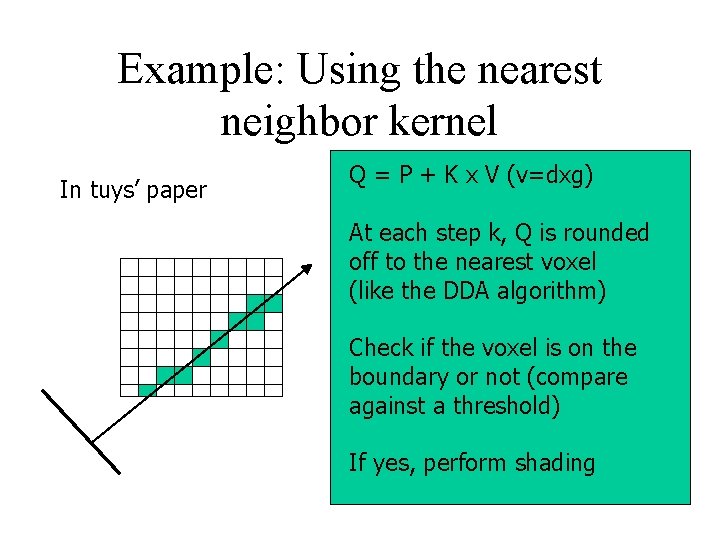
Example: Using the nearest neighbor kernel In tuys’ paper Q = P + K x V (v=dxg) At each step k, Q is rounded off to the nearest voxel (like the DDA algorithm) Check if the voxel is on the boundary or not (compare against a threshold) If yes, perform shading

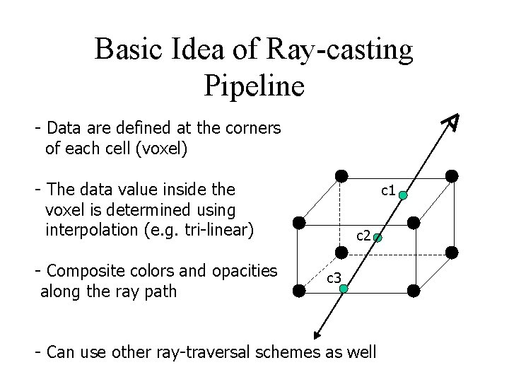
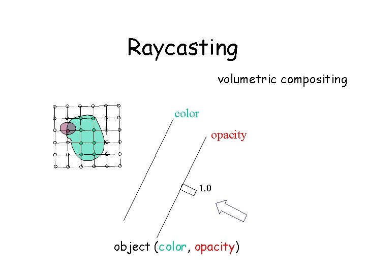
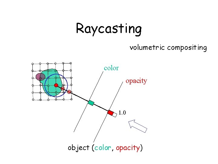
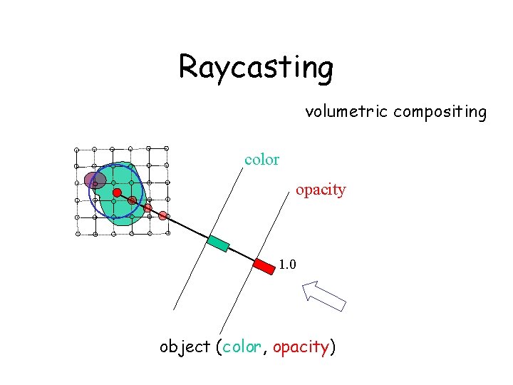
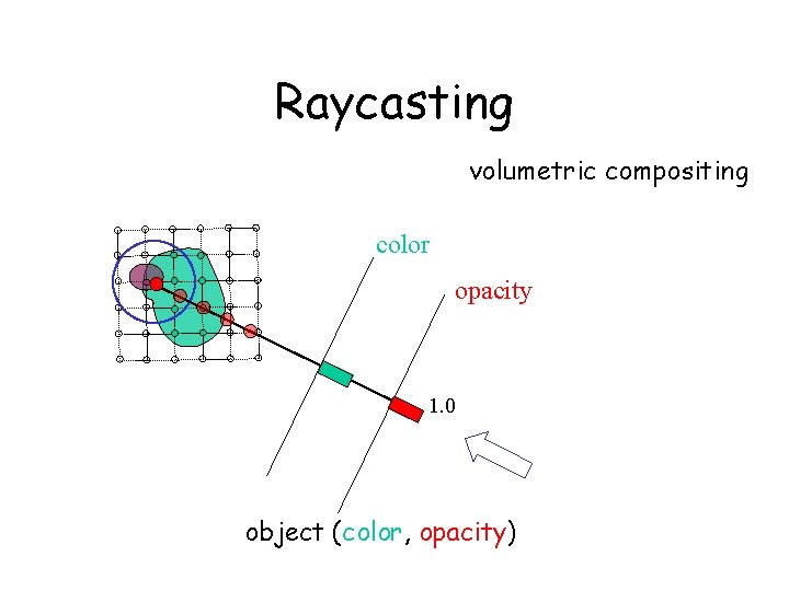
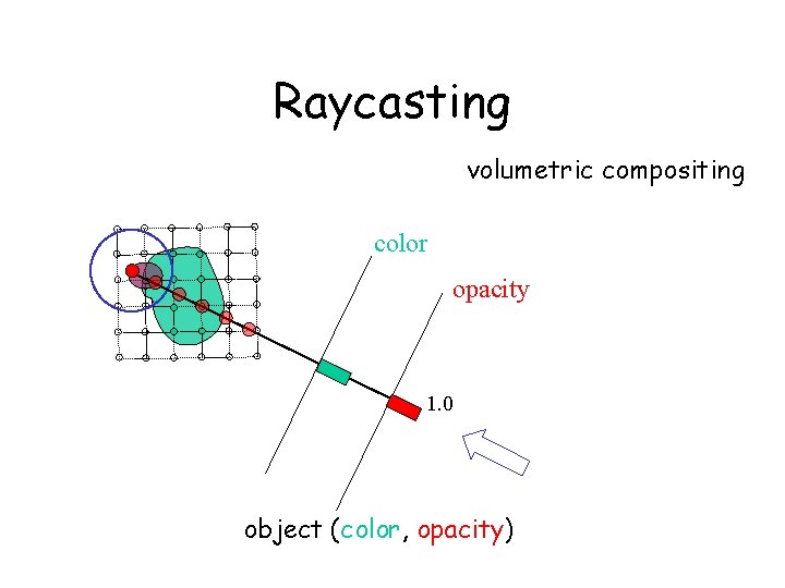
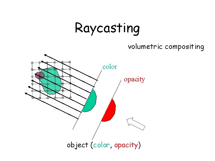
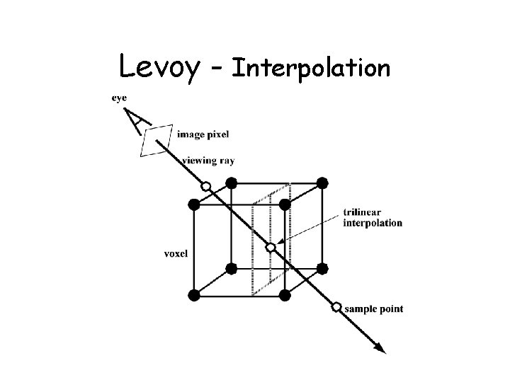
Basic Idea of Ray-casting Pipeline - Data are defined at the corners of each cell (voxel) - The data value inside the voxel is determined using interpolation (e. g. tri-linear) - Composite colors and opacities along the ray path c 1 c 2 c 3 - Can use other ray-traversal schemes as well

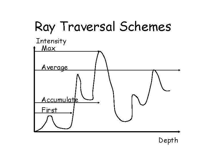
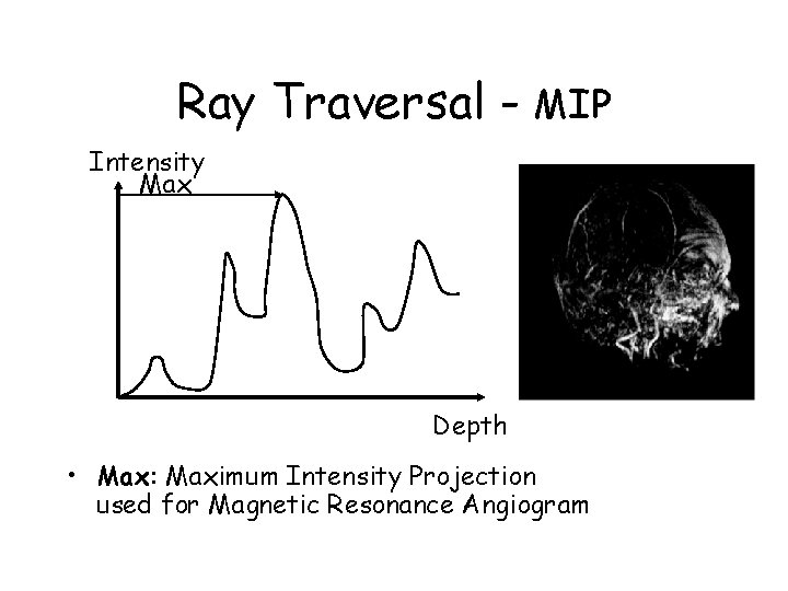
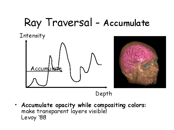
Ray Traversal Schemes Intensity Max Average Accumulate First Depth

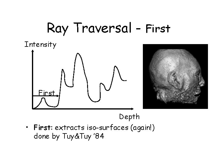
Ray Traversal - First Intensity First Depth • First: extracts iso-surfaces (again!) done by Tuy&Tuy ’ 84

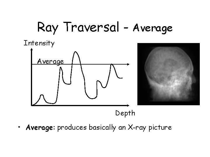
Ray Traversal - Average Intensity Average Depth • Average: produces basically an X-ray picture

Ray Traversal - MIP Intensity Max Depth • Max: Maximum Intensity Projection used for Magnetic Resonance Angiogram

Ray Traversal - Accumulate Intensity Accumulate Depth • Accumulate opacity while compositing colors: make transparent layers visible! Levoy ‘ 88

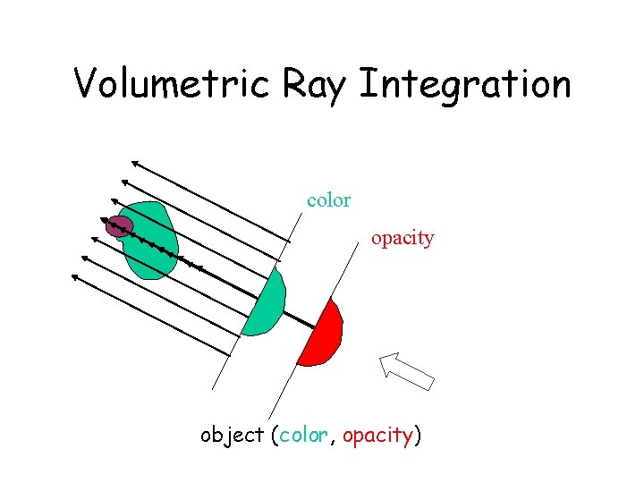
Raycasting volumetric compositing color opacity 1. 0 object (color, opacity)

Raycasting Interpolation kernel volumetric compositing color opacity 1. 0 object (color, opacity)

Raycasting Interpolation kernel volumetric compositing color c = c s s(1 - ) + c opacity = s (1 - ) + 1. 0 object (color, opacity)

Raycasting volumetric compositing color opacity 1. 0 object (color, opacity)

Raycasting volumetric compositing color opacity 1. 0 object (color, opacity)

Raycasting volumetric compositing color opacity 1. 0 object (color, opacity)

Raycasting volumetric compositing color opacity 1. 0 object (color, opacity)

Raycasting volumetric compositing color opacity object (color, opacity)

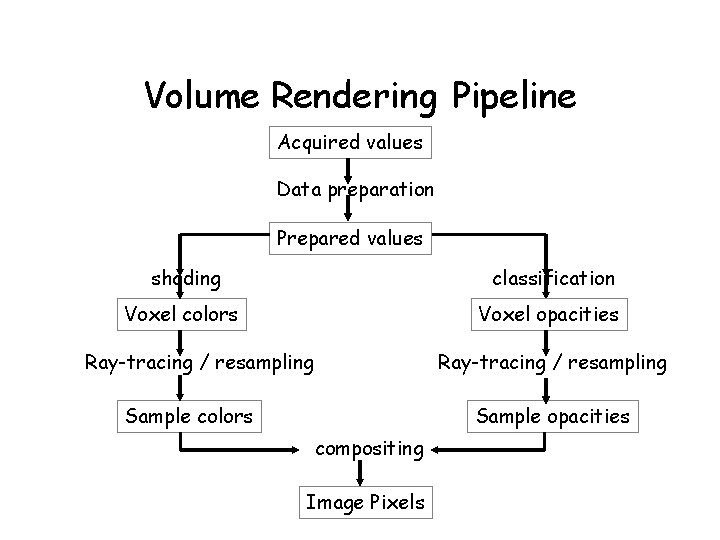
Volume Rendering Pipeline Acquired values Data preparation Prepared values shading classification Voxel colors Voxel opacities Ray-tracing / resampling Sample colors Sample opacities compositing Image Pixels

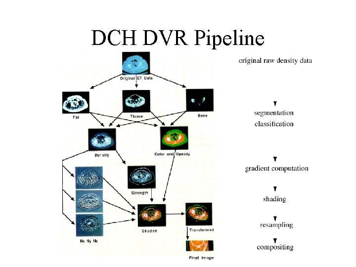
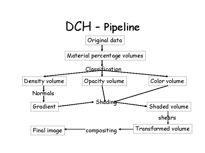
DCH DVR Pipeline

DCH - Pipeline Original data Material percentage volumes Classification Density volume Opacity volume Color volume Normals Gradient Shading Shaded volume shears Final image compositing Transformed volume

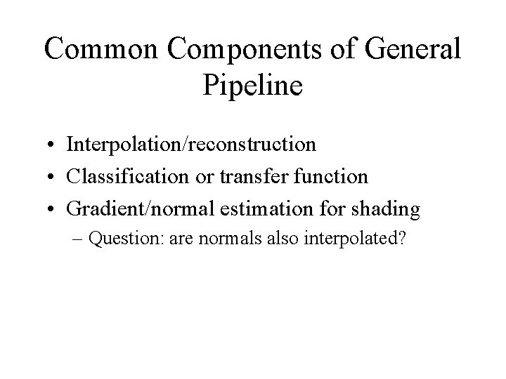
Common Components of General Pipeline • Interpolation/reconstruction • Classification or transfer function • Gradient/normal estimation for shading – Question: are normals also interpolated?

Levoy - Interpolation

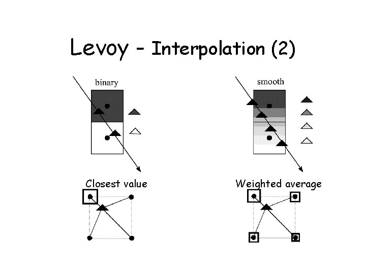
Levoy - Interpolation (2) Closest value Weighted average

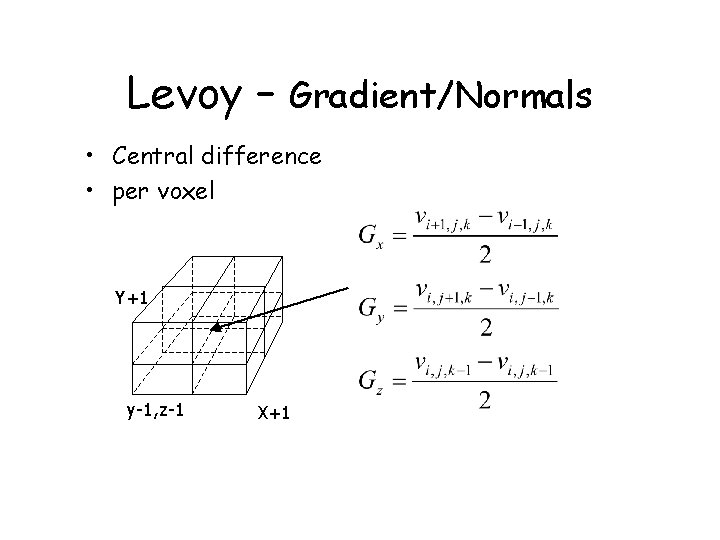
Levoy – Gradient/Normals • Central difference • per voxel Y+1 y-1, z-1 X+1

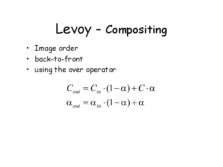
Levoy - Compositing • Image order • back-to-front • using the over operator

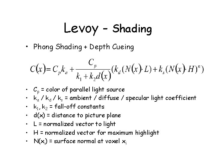
Levoy - Shading • Phong Shading + Depth Cueing • • Cp = color of parallel light source ka / kd / ks = ambient / diffuse / specular light coefficient k 1, k 2 = fall-off constants d(x) = distance to picture plane L = normalized vector to light H = normalized vector for maximum highlight N(xi) = surface normal at voxel xi

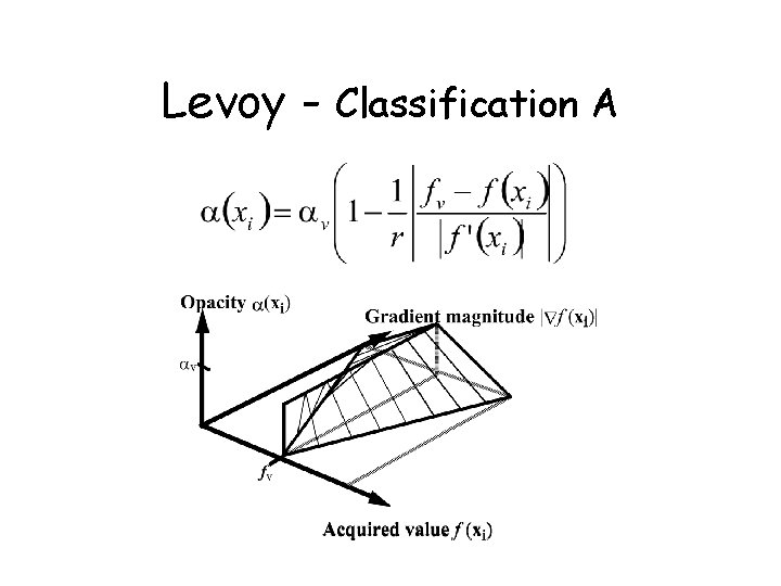
Classification: Mapping from data to opacities Region of interest: high opaicity (more opaque) Rest: translucent or transparent The opacity function is typically specified by the user Levoy came up with two formula to compute opacity 1. Isosurface 2. Region boundary (e. g. between bone and fresh)

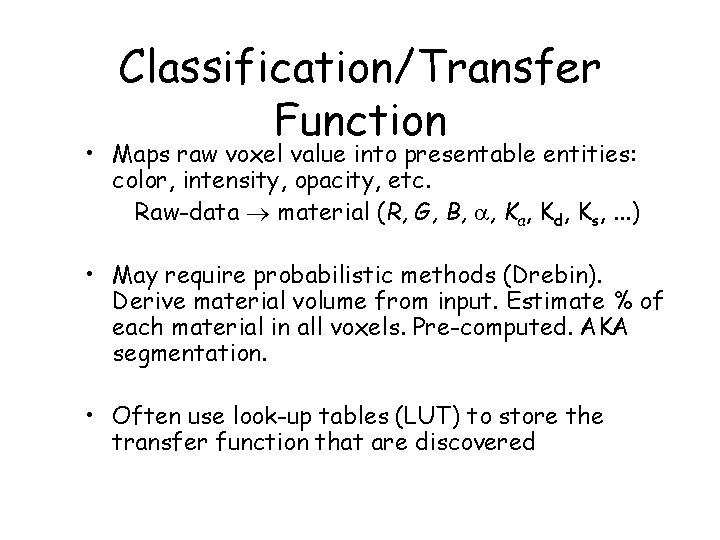
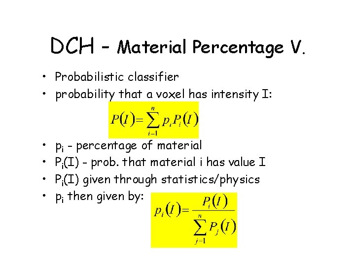
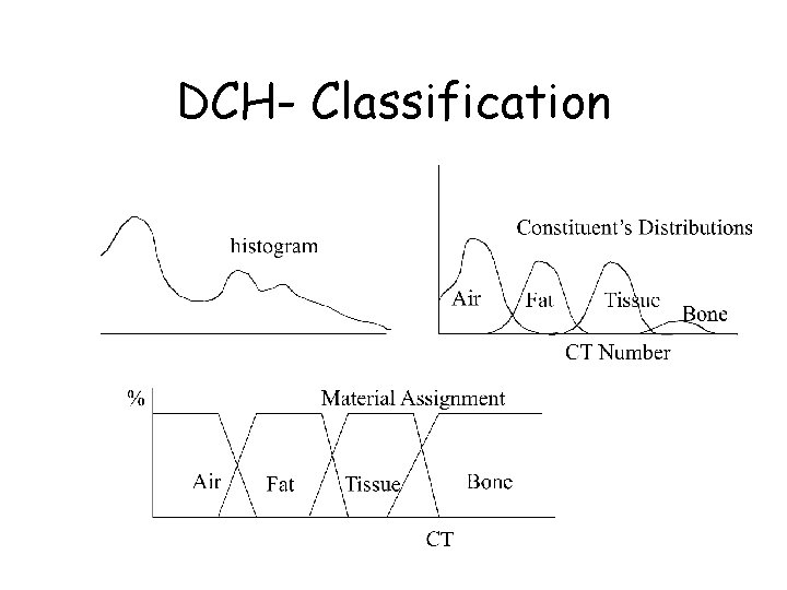
Classification/Transfer Function • Maps raw voxel value into presentable entities: color, intensity, opacity, etc. Raw-data material (R, G, B, , Ka, Kd, Ks, . . . ) • May require probabilistic methods (Drebin). Derive material volume from input. Estimate % of each material in all voxels. Pre-computed. AKA segmentation. • Often use look-up tables (LUT) to store the transfer function that are discovered

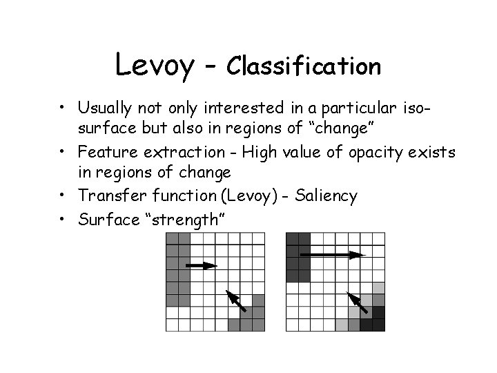
Levoy - Classification • Usually not only interested in a particular isosurface but also in regions of “change” • Feature extraction - High value of opacity exists in regions of change • Transfer function (Levoy) - Saliency • Surface “strength”

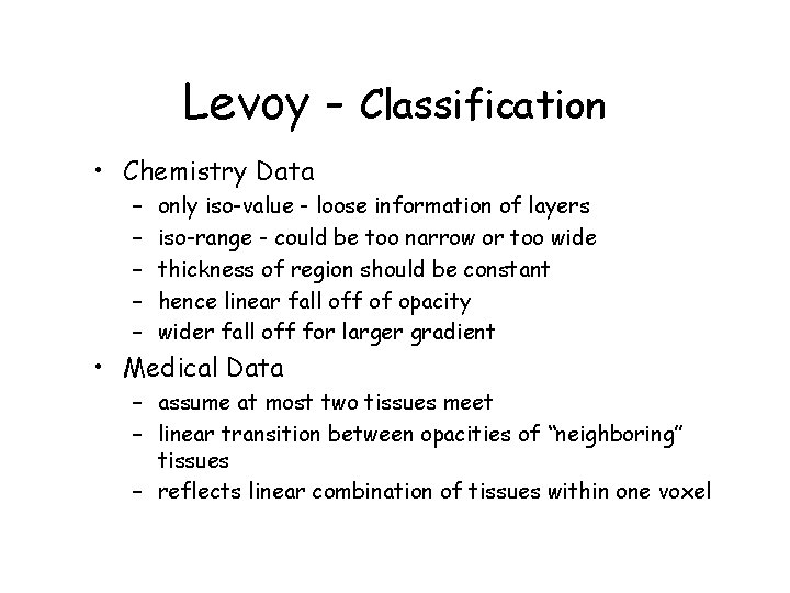
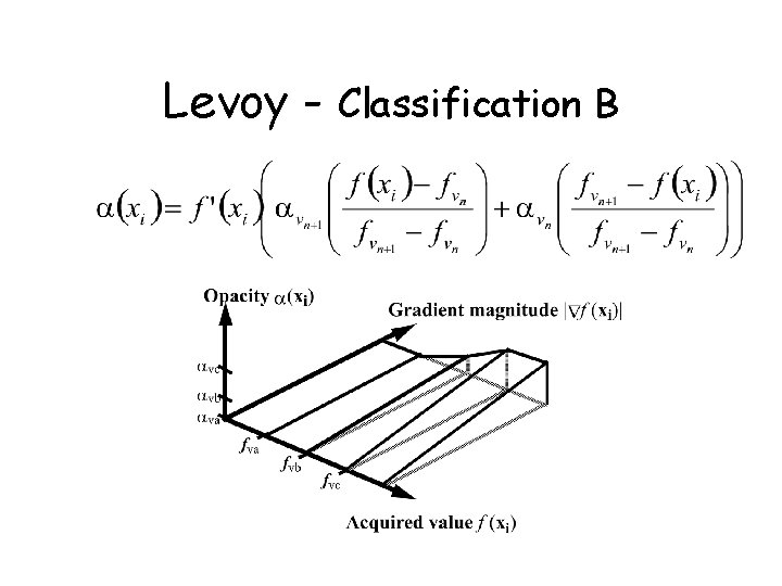
Levoy - Classification • Chemistry Data – – – only iso-value - loose information of layers iso-range - could be too narrow or too wide thickness of region should be constant hence linear fall off of opacity wider fall off for larger gradient • Medical Data – assume at most two tissues meet – linear transition between opacities of “neighboring” tissues – reflects linear combination of tissues within one voxel

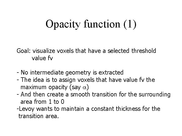
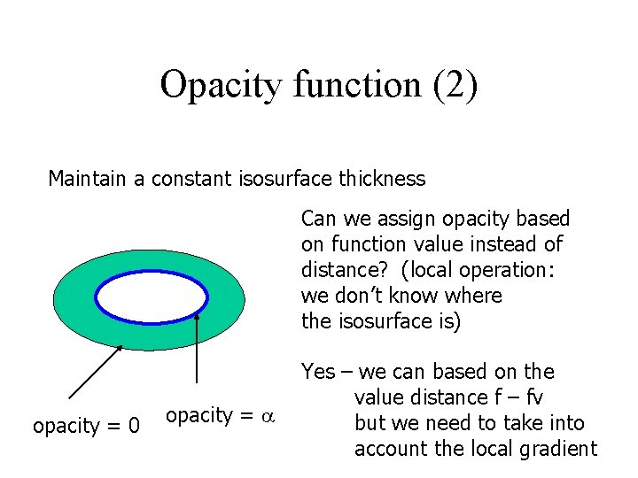
Opacity function (1) Goal: visualize voxels that have a selected threshold value fv - No intermediate geometry is extracted - The idea is to assign voxels that have value fv the maximum opacity (say ) - And then create a smooth transition for the surrounding area from 1 to 0 -Levoy wants to maintain a constant thickness for the transition area.

Opacity function (2) Maintain a constant isosurface thickness Can we assign opacity based on function value instead of distance? (local operation: we don’t know where the isosurface is) opacity = 0 opacity = Yes – we can based on the value distance f – fv but we need to take into account the local gradient

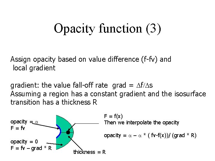
Opacity function (3) Assign opacity based on value difference (f-fv) and local gradient: the value fall-off rate grad = Df/Ds Assuming a region has a constant gradient and the isosurface transition has a thickness R opacity = F = fv opacity = 0 F = fv – grad * R F = f(x) Then we interpolate the opacity = – * ( fv-f(x))/ (grad * R) thickness = R

Levoy - Classification A

Levoy - Classification B

DCH - Material Percentage V. • Probabilistic classifier • probability that a voxel has intensity I: • • pi - percentage of material Pi(I) - prob. that material i has value I Pi(I) given through statistics/physics pi then given by:

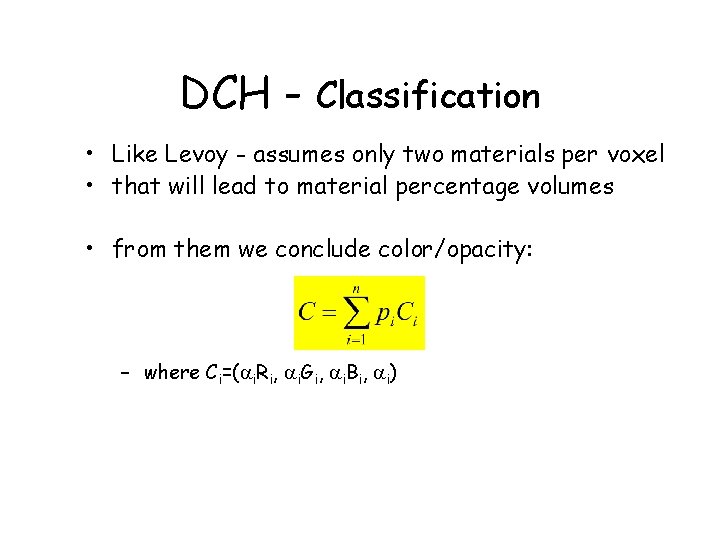
DCH - Classification • Like Levoy - assumes only two materials per voxel • that will lead to material percentage volumes • from them we conclude color/opacity: – where Ci=( i. Ri, i. Gi, i. Bi, i)

DCH- Classification

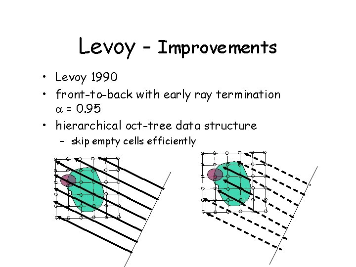
Levoy - Improvements • Levoy 1990 • front-to-back with early ray termination = 0. 95 • hierarchical oct-tree data structure – skip empty cells efficiently

Volumetric Ray Integration color opacity 1. 0 object (color, opacity)