CPCS 391 Computer Graphics 1 Lecture 5 Polygon

+ CPCS 391 Computer Graphics 1 Lecture 5: Polygon Filling Instructor: Dr. Sahar Shabanah

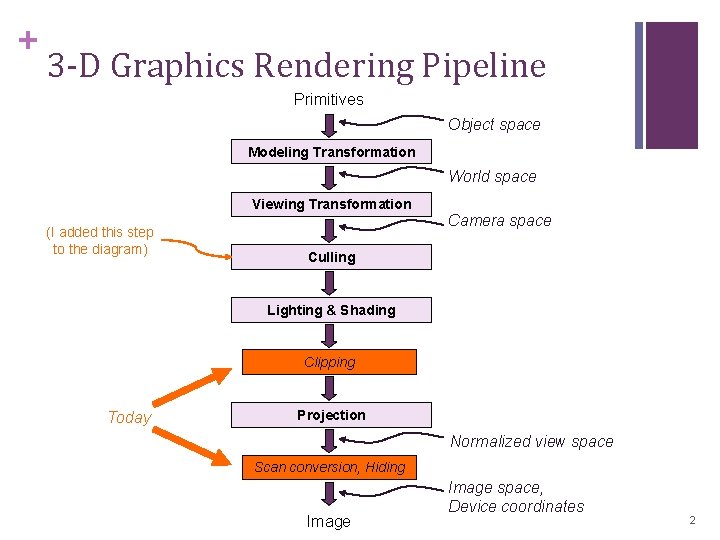
+ 3 -D Graphics Rendering Pipeline Primitives Object space Modeling Transformation World space Viewing Transformation (I added this step to the diagram) Camera space Culling Lighting & Shading Clipping Today Projection Normalized view space Scan conversion, Hiding Image space, Device coordinates 2

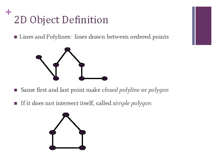
+ 2 D Object Definition n Lines and Polylines: lines drawn between ordered points n Same first and last point make closed polyline or polygon n If it does not intersect itself, called simple polygon

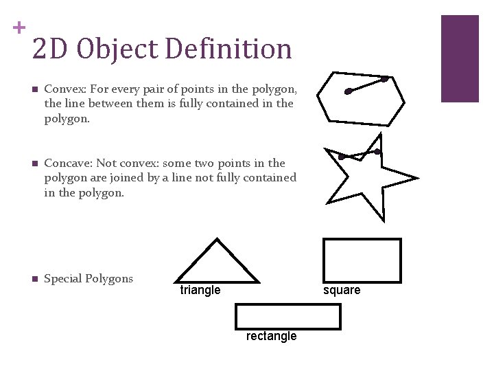
+ 2 D Object Definition n Convex: For every pair of points in the polygon, the line between them is fully contained in the polygon. n Concave: Not convex: some two points in the polygon are joined by a line not fully contained in the polygon. n Special Polygons triangle square rectangle

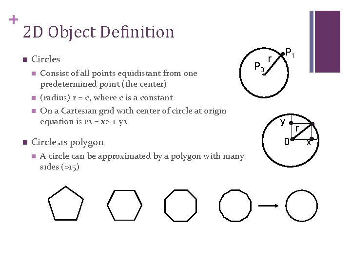
+ 2 D Object Definition n n Circles n Consist of all points equidistant from one predetermined point (the center) n (radius) r = c, where c is a constant n On a Cartesian grid with center of circle at origin equation is r 2 = x 2 + y 2 Circle as polygon n A circle can be approximated by a polygon with many sides (>15) P 0 P 1 r y 0 r x

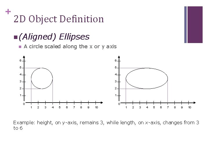
+ 2 D Object Definition n (Aligned) Ellipses n A circle scaled along the x or y axis 6 6 5 5 4 4 3 3 2 2 1 1 0 0 1 2 3 4 5 6 7 8 9 10 Example: height, on y-axis, remains 3, while length, on x-axis, changes from 3 to 6

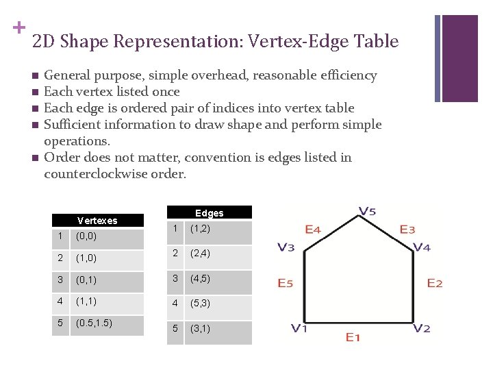
+ 2 D Shape Representation: Vertex-Edge Table n n n General purpose, simple overhead, reasonable efficiency Each vertex listed once Each edge is ordered pair of indices into vertex table Sufficient information to draw shape and perform simple operations. Order does not matter, convention is edges listed in counterclockwise order. Vertexes Edges 1 (1, 2) (1, 0) 2 (2, 4) 3 (0, 1) 3 (4, 5) 4 (1, 1) 4 (5, 3) 5 (0. 5, 1. 5) 5 (3, 1) 1 (0, 0) 2

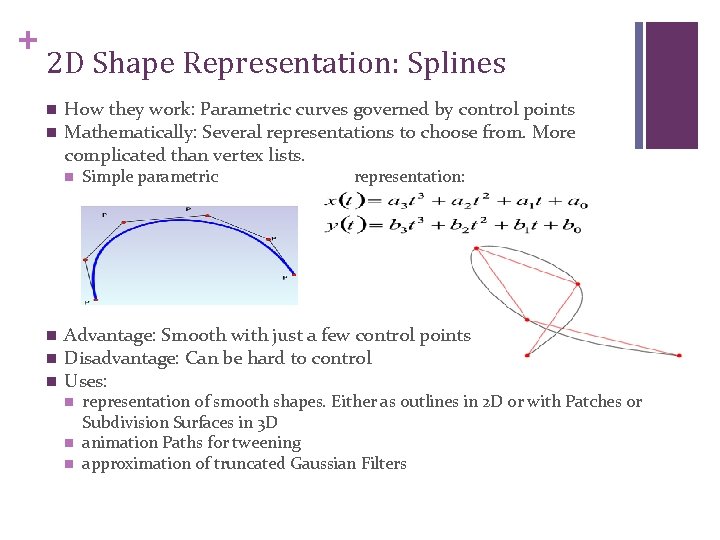
+ 2 D Shape Representation: Splines n n How they work: Parametric curves governed by control points Mathematically: Several representations to choose from. More complicated than vertex lists. n n Simple parametric representation: Advantage: Smooth with just a few control points Disadvantage: Can be hard to control Uses: n n n representation of smooth shapes. Either as outlines in 2 D or with Patches or Subdivision Surfaces in 3 D animation Paths for tweening approximation of truncated Gaussian Filters

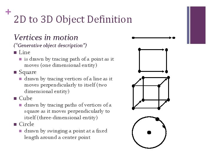
+ 2 D to 3 D Object Definition Vertices in motion (“Generative object description”) n Line n n Square n n drawn by tracing vertices of a line as it moves perpendicularly to itself (two dimensional entity) Cube n n is drawn by tracing path of a point as it moves (one dimensional entity) drawn by tracing paths of vertices of a square as it moves perpendicularly to itself (three-dimensional entity) Circle n drawn by swinging a point at a fixed length around a center point

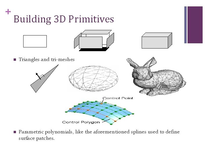
+ Building 3 D Primitives n Triangles and tri-meshes n Parametric polynomials, like the aforementioned splines used to define surface patches.

+ Triangle Meshes n Most common representation of shape in three dimensions n All vertices of triangle are guaranteed to lie in one plane (unlike quadrilaterals or other polygons) n Uniformity makes it easy to perform mesh operations: subdivision, simplification, etc. n Many different ways to represent triangular meshes: http: //en. wikipedia. org/wiki/Polygon_mesh

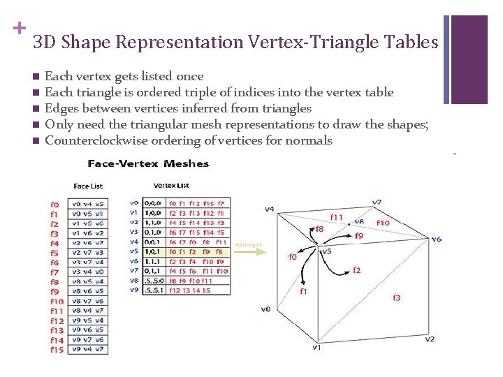
+ 3 D Shape Representation Vertex-Triangle Tables n n n Each vertex gets listed once Each triangle is ordered triple of indices into the vertex table Edges between vertices inferred from triangles Only need the triangular mesh representations to draw the shapes; Counterclockwise ordering of vertices for normals

+ Polygon Fill Algorithms n. A standard output primitive in general graphics package is a solid color or patterned polygon area. n There are two basic approaches to filling on raster systems. Scan line polygon fill: determine overlap Intervals for scan lines that cross that area, mostly used in general graphics packages n Seed fill: start from a given interior point and paint outward from this point until we encounter the boundary, used in applications having complex boundaries and interactive painting systems n

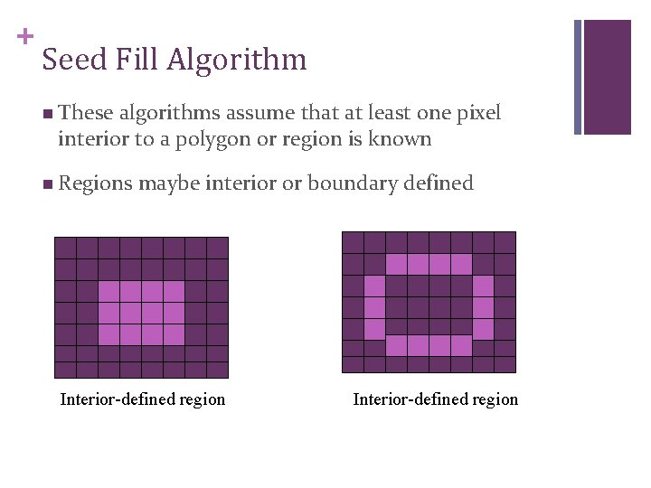
+ Seed Fill Algorithm n These algorithms assume that at least one pixel interior to a polygon or region is known n Regions maybe interior or boundary defined Interior-defined region

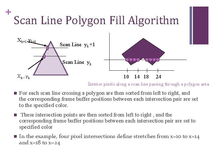
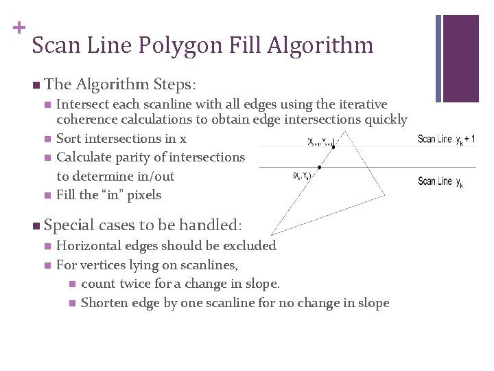
+ Scan Line Polygon Fill Algorithm Xk+1, yk+1 Scan Line yk Xk , yk 10 14 18 24 Interior pixels along a scan line passing through a polygon area n For each scan line crossing a polygon are then sorted from left to right, and the corresponding frame buffer positions between each intersection pair are set to the specified color. n These intersection points are then sorted from left to right , and the corresponding frame buffer positions between each intersection pair are set to specified color n In the example, four pixel intersections define stretches from x=10 to x=14 and x=18 to x=24

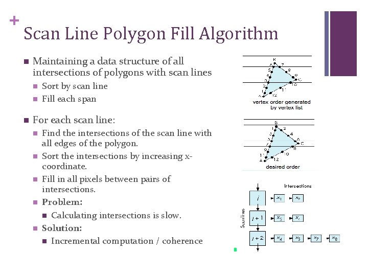
+ Scan Line Polygon Fill Algorithm n Maintaining a data structure of all intersections of polygons with scan lines n n n Sort by scan line Fill each span For each scan line: n n n Find the intersections of the scan line with all edges of the polygon. Sort the intersections by increasing xcoordinate. Fill in all pixels between pairs of intersections. Problem: n Calculating intersections is slow. Solution: n Incremental computation / coherence

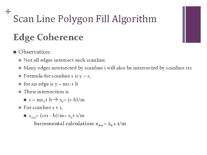
+ Scan Line Polygon Fill Algorithm Edge Coherence n Observation: n Not all edges intersect each scanline. n Many edges intersected by scanline i will also be intersected by scanline i+1 n Formula for scanline s is y = s, n for an edge is y = mx + b n Their intersection is n n s = mxs+ b xs= (s-b)/m For scanline s + 1, n xs+1= (s+1 - b)/m= xs+ 1/m Incremental calculation: xs+1 = xs + 1/m

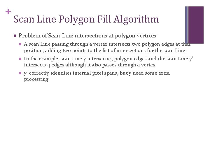
+ Scan Line Polygon Fill Algorithm n Problem of Scan-Line intersections at polygon vertices: n A scan Line passing through a vertex intersects two polygon edges at that position, adding two points to the list of intersections for the scan Line n In the example, scan Line y intersects 5 polygon edges and the scan Line y‘ intersects 4 edges although it also passes through a vertex n y‘ correctly identifies internal pixel spans, but y need some extra processing

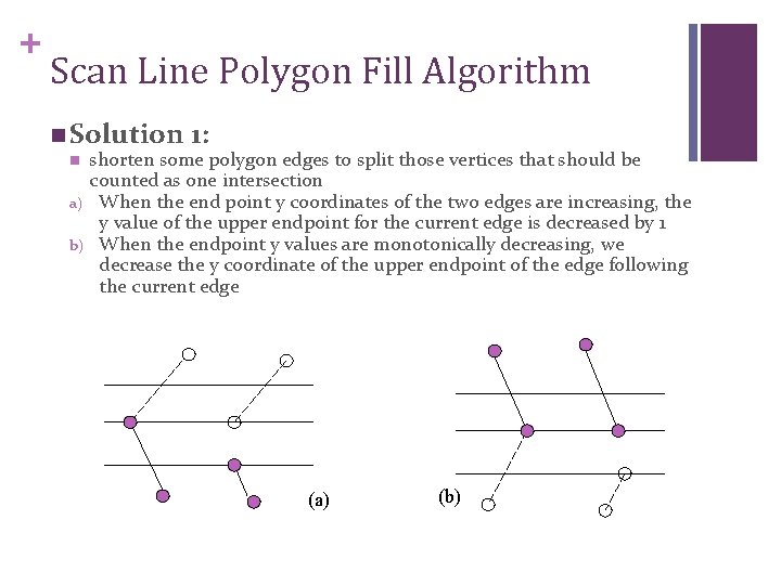
+ Scan Line Polygon Fill Algorithm n Solution 1: shorten some polygon edges to split those vertices that should be counted as one intersection a) When the end point y coordinates of the two edges are increasing, the y value of the upper endpoint for the current edge is decreased by 1 b) When the endpoint y values are monotonically decreasing, we decrease the y coordinate of the upper endpoint of the edge following the current edge n (a) (b)

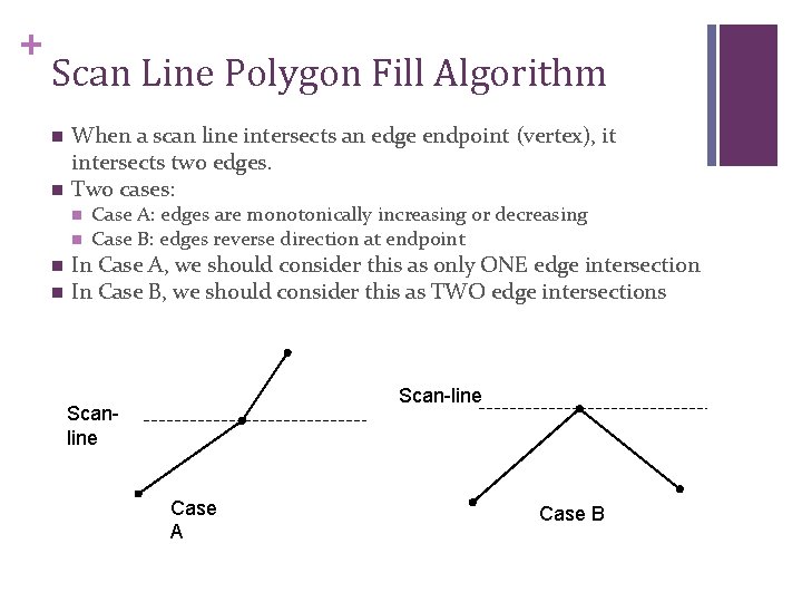
+ Scan Line Polygon Fill Algorithm n n When a scan line intersects an edge endpoint (vertex), it intersects two edges. Two cases: n n Case A: edges are monotonically increasing or decreasing Case B: edges reverse direction at endpoint In Case A, we should consider this as only ONE edge intersection In Case B, we should consider this as TWO edge intersections Scan-line Scanline Case A Case B

+ Scan Line Polygon Fill Algorithm n The n n Algorithm Steps: Intersect each scanline with all edges using the iterative coherence calculations to obtain edge intersections quickly Sort intersections in x Calculate parity of intersections to determine in/out Fill the “in” pixels n Special n n cases to be handled: Horizontal edges should be excluded For vertices lying on scanlines, n count twice for a change in slope. n Shorten edge by one scanline for no change in slope

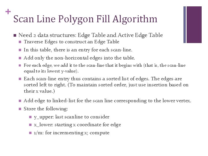
+ Scan Line Polygon Fill Algorithm n Need 2 data structures: Edge Table and Active Edge Table n Traverse Edges to construct an Edge Table n In this table, there is an entry for each scan-line. n Add only the non-horizontal edges into the table. n For each edge, we add it to the scan-line that it begins with (that is, the scan-line equal to its lowest y-value). n Each scan-line entry thus contains a sorted list of edges. The edges are sorted left to right. (To maintain sorted order, just use insertion based on their x value. ) n Add edge to linked-list for the scan line corresponding to the lower vertex. n Store the following: n y_upper: last scanline to consider n x_lower: starting x coordinate for edge n 1/m: for incrementing x; compute

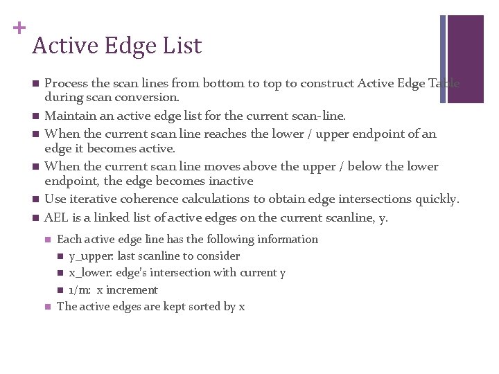
+ Active Edge List n n n Process the scan lines from bottom to top to construct Active Edge Table during scan conversion. Maintain an active edge list for the current scan-line. When the current scan line reaches the lower / upper endpoint of an edge it becomes active. When the current scan line moves above the upper / below the lower endpoint, the edge becomes inactive Use iterative coherence calculations to obtain edge intersections quickly. AEL is a linked list of active edges on the current scanline, y. n n Each active edge line has the following information n y_upper: last scanline to consider n x_lower: edge’s intersection with current y n 1/m: x increment The active edges are kept sorted by x

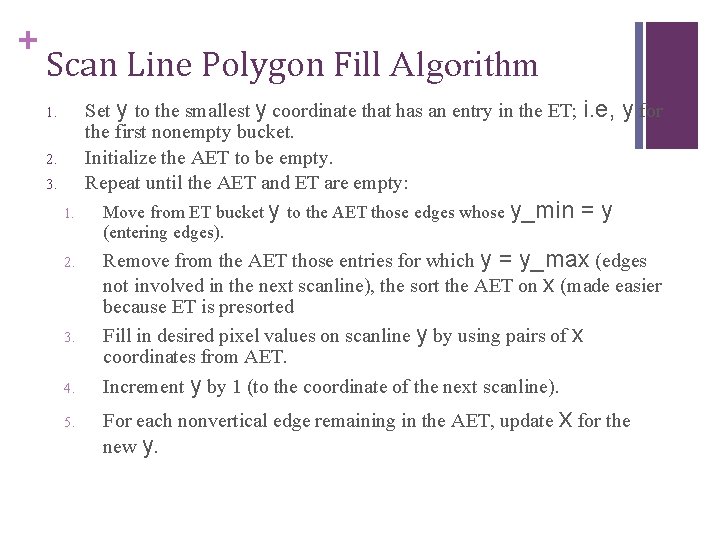
+ Scan Line Polygon Fill Algorithm Set y to the smallest y coordinate that has an entry in the ET; i. e, the first nonempty bucket. Initialize the AET to be empty. Repeat until the AET and ET are empty: 1. 2. 3. 1. 2. 3. 4. 5. Move from ET bucket y to the AET those edges whose y_min (entering edges). y for =y Remove from the AET those entries for which y = y_max (edges not involved in the next scanline), the sort the AET on x (made easier because ET is presorted Fill in desired pixel values on scanline y by using pairs of x coordinates from AET. Increment y by 1 (to the coordinate of the next scanline). For each nonvertical edge remaining in the AET, update x for the new y.

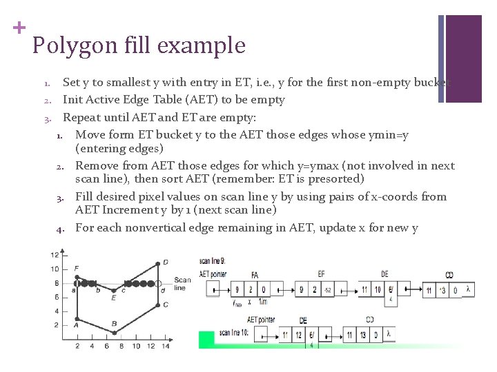
+ Polygon fill example 1. 2. 3. Set y to smallest y with entry in ET, i. e. , y for the first non-empty bucket Init Active Edge Table (AET) to be empty Repeat until AET and ET are empty: 1. Move form ET bucket y to the AET those edges whose ymin=y (entering edges) 2. Remove from AET those edges for which y=ymax (not involved in next scan line), then sort AET (remember: ET is presorted) 3. Fill desired pixel values on scan line y by using pairs of x-coords from AET Increment y by 1 (next scan line) 4. For each nonvertical edge remaining in AET, update x for new y

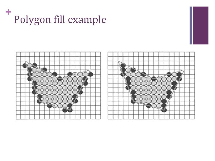
+ Polygon fill example