Computing for Scientists Scientific Simulation SS Sep 27

Computing for Scientists Scientific Simulation (SS) (Sep. 27, 2011 – TBD) Jie Zhang Copyright © CDS 130 - 001 Fall, 2011

Contents 1. Introduction 2. Mathematical Models 3. Computational Models 3. 1. Basics: Algorithm, Iteration, Interval. Subinterval 3. 2. Differentiation 3. 3. Integration 4. Scientific Method

SS-1: Introduction (Sep. 27, 2011)

Motivation • Scientific simulation allows one to produce the details and predict the behavior of a complex scientific system, e. g. , physical systems, engineering systems, biological systems, environmental systems etc. • It is a new way of scientific research, in additional to traditional experimental (including observations) and mathematical approaches.

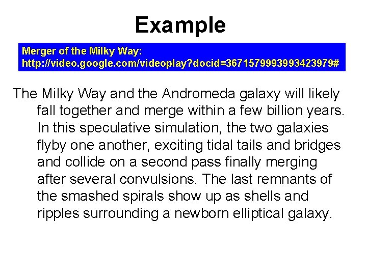
Example Merger of the Milky Way: http: //video. google. com/videoplay? docid=3671579993993423979# The Milky Way and the Andromeda galaxy will likely fall together and merge within a few billion years. In this speculative simulation, the two galaxies flyby one another, exciting tidal tails and bridges and collide on a second pass finally merging after several convulsions. The last remnants of the smashed spirals show up as shells and ripples surrounding a newborn elliptical galaxy.

Example Cellular Blood Flow: http: //www. youtube. com/watch? v=o 11 NDvr. ZMNs&feature=related The RBCs are modeled as a membrane with hemoglobin inside with a viscosity of 6 c. P. Each RBC membrane is constructed of linear finite element� triangular shells. These shell elements deform due to the fluid-structure interactions with the blood plasma and the hemoglobin.

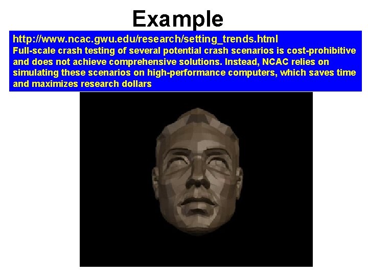
Example http: //www. ncac. gwu. edu/research/setting_trends. html Full-scale crash testing of several potential crash scenarios is cost-prohibitive and does not achieve comprehensive solutions. Instead, NCAC relies on simulating these scenarios on high-performance computers, which saves time and maximizes research dollars

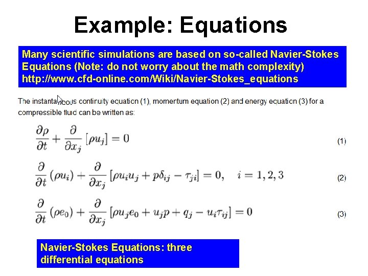
Example: Equations Many scientific simulations are based on so-called Navier-Stokes Equations (Note: do not worry about the math complexity) http: //www. cfd-online. com/Wiki/Navier-Stokes_equations Navier-Stokes Equations: three differential equations

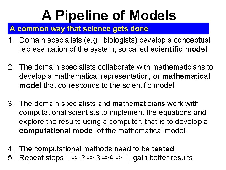
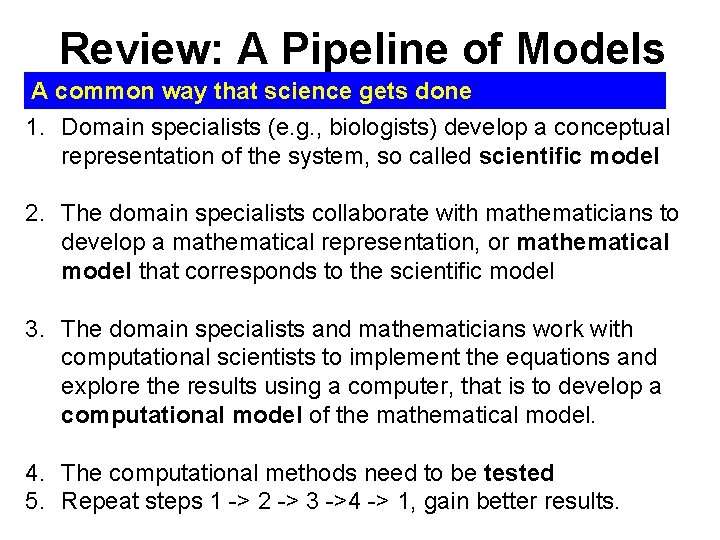
A Pipeline of Models A common way that science gets done 1. Domain specialists (e. g. , biologists) develop a conceptual representation of the system, so called scientific model 2. The domain specialists collaborate with mathematicians to develop a mathematical representation, or mathematical model that corresponds to the scientific model 3. The domain specialists and mathematicians work with computational scientists to implement the equations and explore the results using a computer, that is to develop a computational model of the mathematical model. 4. The computational methods need to be tested 5. Repeat steps 1 -> 2 -> 3 ->4 -> 1, gain better results.

SS-2: Mathematical Models (Sep. 29, 2011)

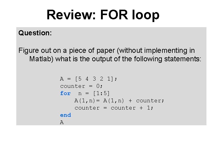
Review: FOR loop Question: Figure out on a piece of paper (without implementing in Matlab) what is the output of the following statements: A = [5 4 3 2 1]; counter = 0; for n = [1: 5] A(1, n)= A(1, n) + counter; counter = counter + 1; end A

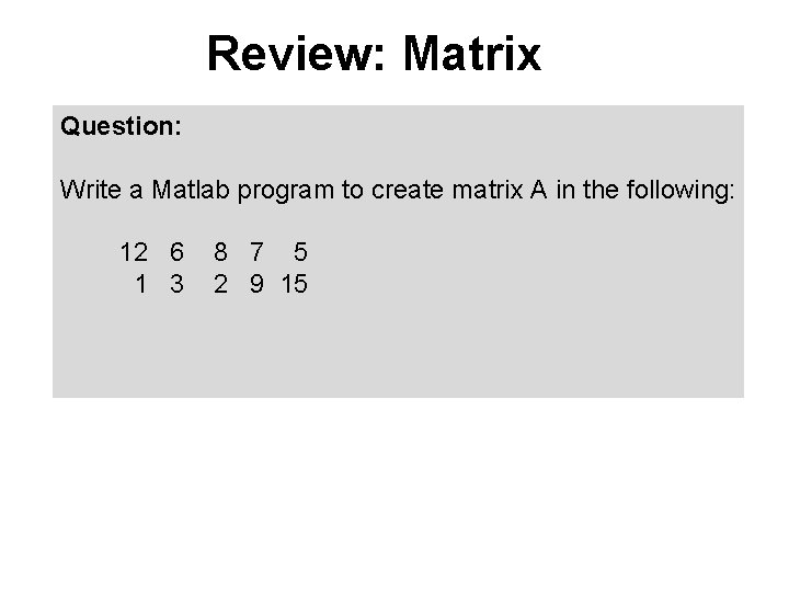
Review: Matrix Question: Write a Matlab program to create matrix A in the following: 12 6 1 3 8 7 5 2 9 15

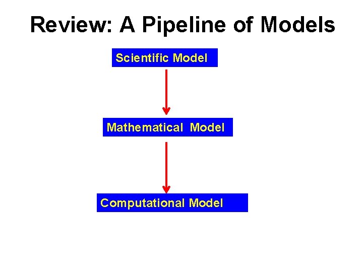
Review: A Pipeline of Models A common way that science gets done 1. Domain specialists (e. g. , biologists) develop a conceptual representation of the system, so called scientific model 2. The domain specialists collaborate with mathematicians to develop a mathematical representation, or mathematical model that corresponds to the scientific model 3. The domain specialists and mathematicians work with computational scientists to implement the equations and explore the results using a computer, that is to develop a computational model of the mathematical model. 4. The computational methods need to be tested 5. Repeat steps 1 -> 2 -> 3 ->4 -> 1, gain better results.

Review: A Pipeline of Models Scientific Model Mathematical Model Computational Model

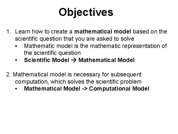
Objectives 1. Learn how to create a mathematical model based on the scientific question that you are asked to solve • Mathematic model is the mathematic representation of the scientific question • Scientific Model Mathematical Model 2. Mathematical model is necessary for subsequent computation, which solves the scientific problem • Mathematical Model -> Computational Model

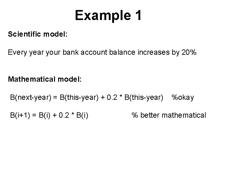
Example 1 Scientific model: Every year your bank account balance increases by 20% Mathematical model: B(next-year) = B(this-year) + 0. 2 * B(this-year) B(i+1) = B(i) + 0. 2 * B(i) %okay % better mathematical

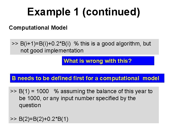
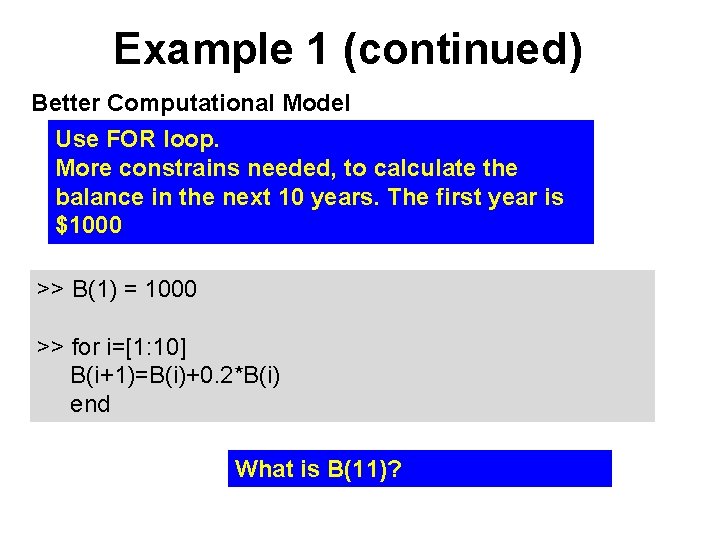
Example 1 (continued) Computational Model >> B(i+1)=B(i)+0. 2*B(i) % this is a good algorithm, but not good implementation What is wrong with this? B needs to be defined first for a computational model >> B(1) = 1000 % assuming the balance of this year to be 1000, or any input number specified by the question >> B(2)=B(2)+0. 2*B(1)

Example 1 (continued) Better Computational Model Use FOR loop. More constrains needed, to calculate the balance in the next 10 years. The first year is $1000 >> B(1) = 1000 >> for i=[1: 10] B(i+1)=B(i)+0. 2*B(i) end What is B(11)?

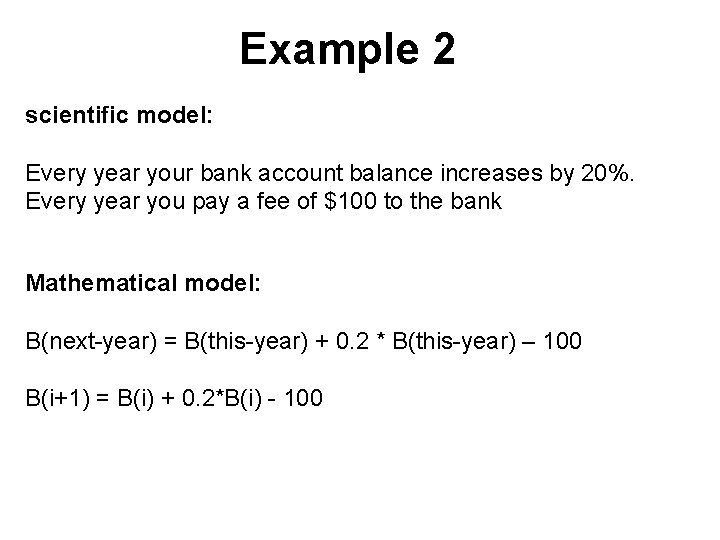
Example 2 scientific model: Every year your bank account balance increases by 20%. Every year you pay a fee of $100 to the bank Mathematical model: B(next-year) = B(this-year) + 0. 2 * B(this-year) – 100 B(i+1) = B(i) + 0. 2*B(i) - 100

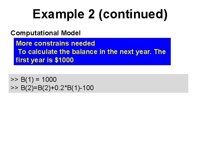
Example 2 (continued) Computational Model More constrains needed To calculate the balance in the next year. The first year is $1000 >> B(1) = 1000 >> B(2)=B(2)+0. 2*B(1)-100

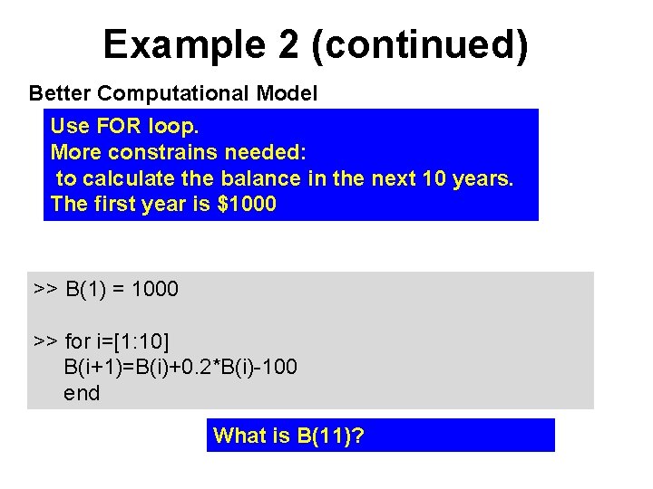
Example 2 (continued) Better Computational Model Use FOR loop. More constrains needed: to calculate the balance in the next 10 years. The first year is $1000 >> B(1) = 1000 >> for i=[1: 10] B(i+1)=B(i)+0. 2*B(i)-100 end What is B(11)?

Example 3 scientific model: Every year your bank account balance doubles. Question: What is the mathematical model?

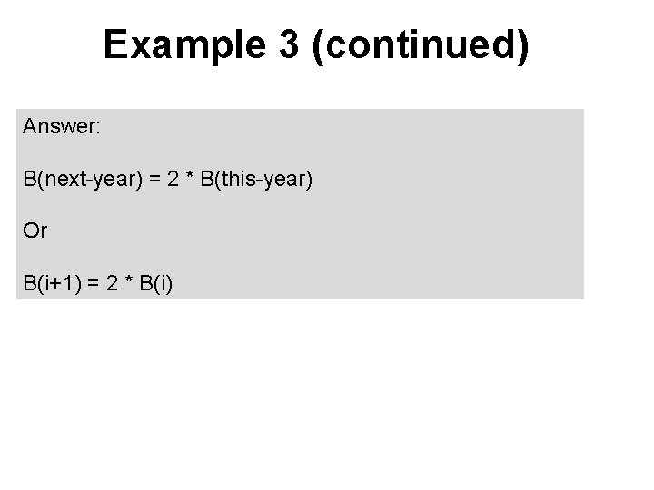
Example 3 (continued) Answer: B(next-year) = 2 * B(this-year) Or B(i+1) = 2 * B(i)

Example 3 (continued) scientific model: Every year your bank account balance doubles. Question: Assuming in the first year, the balance is $1000. Develop a computational model in Matlab to calculate the balance in the next 10 years? What is the balance in the 11 th year?

Example 3 (continued) Answer: >> clear %clear the existing variables >>B(1)=1000 >>for i=[1: 10] B(i+1)=B(i)*2 end >>B(11) Ans = 1024000

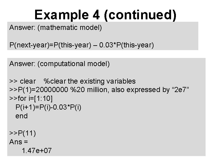
Example 4 scientific model: The death rate of the population in a country suffering from war is 3% per year and no babies are born Question: What is the mathematical model? Question: Develop a computational model to calculate the population in the next 10 years? What is population in the 11 th year? Assuming the initial population is 20 million.

Example 4 (continued) Answer: (mathematic model) P(next-year)=P(this-year) – 0. 03*P(this-year) Answer: (computational model) >> clear %clear the existing variables >>P(1)=20000000 %20 million, also expressed by “ 2 e 7” >>for i=[1: 10] P(i+1)=P(i)-0. 03*P(i) end >>P(11) Ans = 1. 47 e+07

(Sep. 29, 2011 Stops Here)

(Oct. 04, 2011 Starts Here)

SS-2: Mathematical Models (Continued) Predator – Prey Model (Oct. 04, 2011)

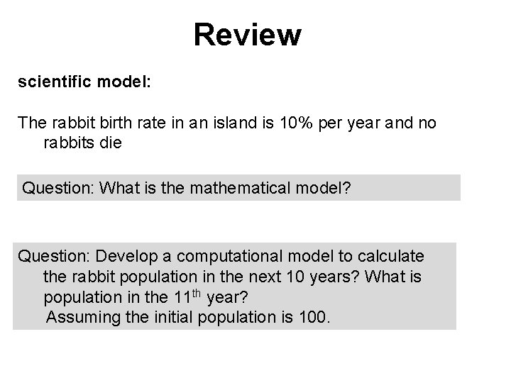
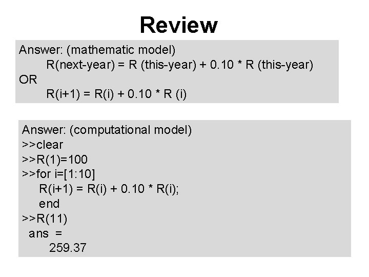
Review scientific model: The rabbit birth rate in an island is 10% per year and no rabbits die Question: What is the mathematical model? Question: Develop a computational model to calculate the rabbit population in the next 10 years? What is population in the 11 th year? Assuming the initial population is 100.

Review Answer: (mathematic model) R(next-year) = R (this-year) + 0. 10 * R (this-year) OR R(i+1) = R(i) + 0. 10 * R (i) Answer: (computational model) >>clear >>R(1)=100 >>for i=[1: 10] R(i+1) = R(i) + 0. 10 * R(i); end >>R(11) ans = 259. 37

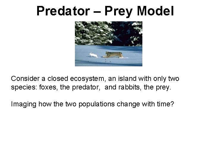
Predator – Prey Model Consider a closed ecosystem, an island with only two species: foxes, the predator, and rabbits, the prey. Imaging how the two populations change with time?

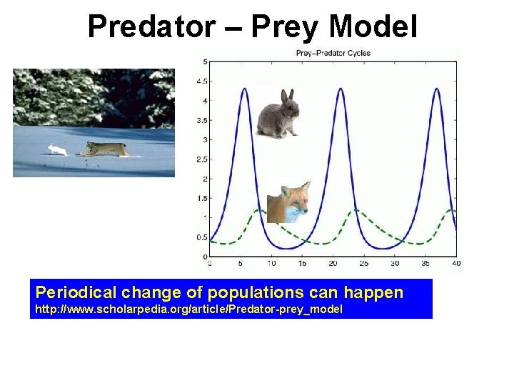
Predator – Prey Model Periodical change of populations can happen http: //www. scholarpedia. org/article/Predator-prey_model

Predator – Prey Model What if the predators are so greedy? What if the preys are so easy to grow?

Predator – Prey Model “Predator-prey models are arguably the building blocks of the bio- and ecosystems as biomasses are grown out of their resource masses. Species compete, evolve and disperse simply for the purpose of seeking resources to sustain their struggle for their very existence. Depending on their specific settings of applications, they can take the forms of resource-consumer, plantherbivore, parasite-host, tumor cells (virus)-immune system, susceptible-infectious interactions, etc. ” (http: //www. scholarpedia. org/article/Predator-prey_model) An online simulator: http: //home. messiah. edu/~deroos/CSC 171/Pred. Prey/PRED. htm

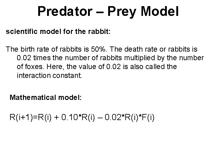
Predator – Prey Model scientific model for the rabbit: The birth rate of rabbits is 50%. The death rate or rabbits is 0. 02 times the number of rabbits multiplied by the number of foxes. Here, the value of 0. 02 is also called the interaction constant. Mathematical model: R(i+1)=R(i) + 0. 10*R(i) – 0. 02*R(i)*F(i)

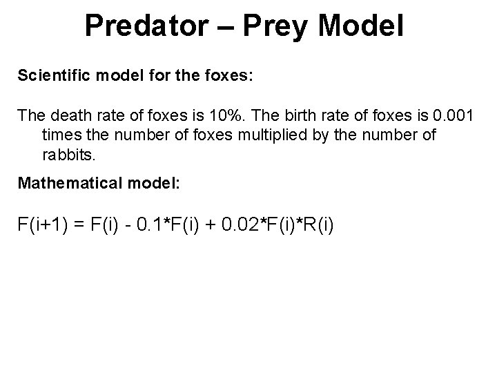
Predator – Prey Model Scientific model for the foxes: The death rate of foxes is 10%. The birth rate of foxes is 0. 001 times the number of foxes multiplied by the number of rabbits. Mathematical model: F(i+1) = F(i) - 0. 1*F(i) + 0. 02*F(i)*R(i)

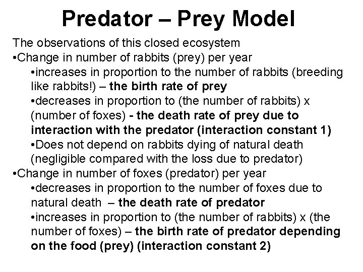
Predator – Prey Model The observations of this closed ecosystem • Change in number of rabbits (prey) per year • increases in proportion to the number of rabbits (breeding like rabbits!) – the birth rate of prey • decreases in proportion to (the number of rabbits) x (number of foxes) - the death rate of prey due to interaction with the predator (interaction constant 1) • Does not depend on rabbits dying of natural death (negligible compared with the loss due to predator) • Change in number of foxes (predator) per year • decreases in proportion to the number of foxes due to natural death – the death rate of predator • increases in proportion to (the number of rabbits) x (the number of foxes) – the birth rate of predator depending on the food (prey) (interaction constant 2)

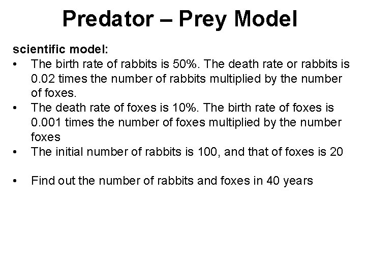
Predator – Prey Model scientific model: • The birth rate of rabbits is 50%. The death rate or rabbits is 0. 02 times the number of rabbits multiplied by the number of foxes. • The death rate of foxes is 10%. The birth rate of foxes is 0. 001 times the number of foxes multiplied by the number foxes • The initial number of rabbits is 100, and that of foxes is 20 • Find out the number of rabbits and foxes in 40 years

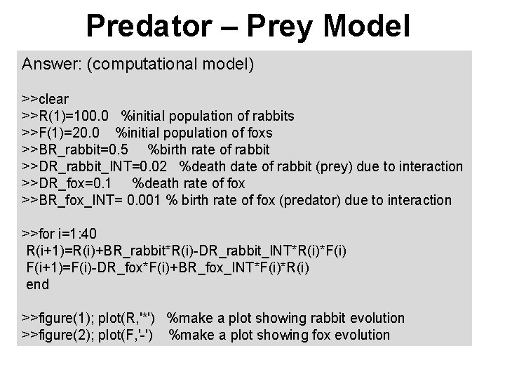
Predator – Prey Model Answer: (computational model) >>clear >>R(1)=100. 0 %initial population of rabbits >>F(1)=20. 0 %initial population of foxs >>BR_rabbit=0. 5 %birth rate of rabbit >>DR_rabbit_INT=0. 02 %death date of rabbit (prey) due to interaction >>DR_fox=0. 1 %death rate of fox >>BR_fox_INT= 0. 001 % birth rate of fox (predator) due to interaction >>for i=1: 40 R(i+1)=R(i)+BR_rabbit*R(i)-DR_rabbit_INT*R(i)*F(i) F(i+1)=F(i)-DR_fox*F(i)+BR_fox_INT*F(i)*R(i) end >>figure(1); plot(R, '*') %make a plot showing rabbit evolution >>figure(2); plot(F, '-') %make a plot showing fox evolution

Predator – Prey Model Practical problems with previous approach 1. It is not convenient to type multiple line programming codes in the command line. Any mistake means re-typing 2. To find the evolution, one needs to use a graphic plot to illustrate the evolution. The plot needs to be well annotated. Sharpen your MATLAB skill

(Oct. 04, 2011 Stops Here)

(Oct. 06, 2011 Starts Here)

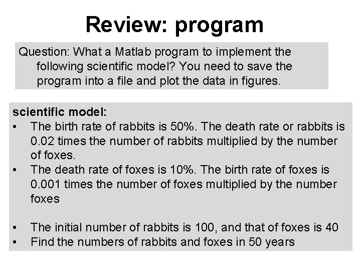
Review: program Question: What a Matlab program to implement the following scientific model? You need to save the program into a file and plot the data in figures. scientific model: • The birth rate of rabbits is 50%. The death rate or rabbits is 0. 02 times the number of rabbits multiplied by the number of foxes. • The death rate of foxes is 10%. The birth rate of foxes is 0. 001 times the number of foxes multiplied by the number foxes • • The initial number of rabbits is 100, and that of foxes is 40 Find the numbers of rabbits and foxes in 50 years

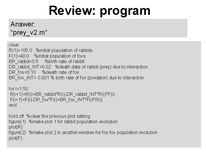
Review: program Answer: “prey_v 2. m” clear R(1)=100. 0 %initial population of rabbits F(1)=40. 0 %initial population of foxs BR_rabbit=0. 5 %birth rate of rabbit DR_rabbit_INT=0. 02 %death date of rabbit (prey) due to interaction DR_fox=0. 10 %death rate of fox BR_fox_INT= 0. 001 % birth rate of fox (predator) due to interaction for i=1: 50 R(i+1)=R(i)+BR_rabbit*R(i)-DR_rabbit_INT*R(i)*F(i) F(i+1)=F(i)-DR_fox*F(i)+BR_fox_INT*F(i)*R(i) end hold off %clear the previous plot setting figure(1) %make plot 1 for rabbit population evolution plot(R) figure(2) %make plot 2 in another window for fox population evolution plot(F)

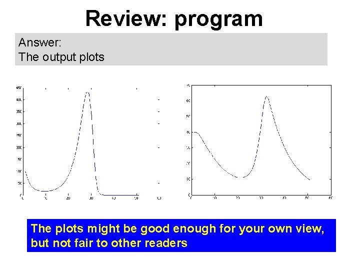
Review: program Answer: The output plots The plots might be good enough for your own view, but not fair to other readers

Matlab (advanced) “plot” function (Oct. 06, 2011)

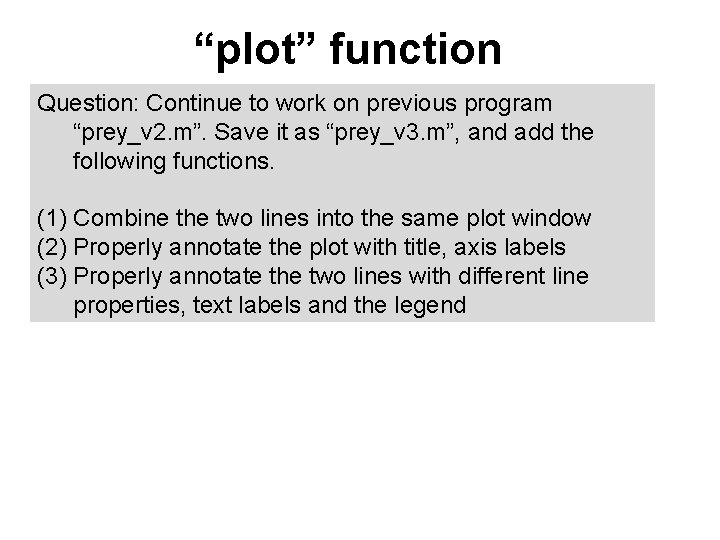
“plot” function Question: Continue to work on previous program “prey_v 2. m”. Save it as “prey_v 3. m”, and add the following functions. (1) Combine the two lines into the same plot window (2) Properly annotate the plot with title, axis labels (3) Properly annotate the two lines with different line properties, text labels and the legend

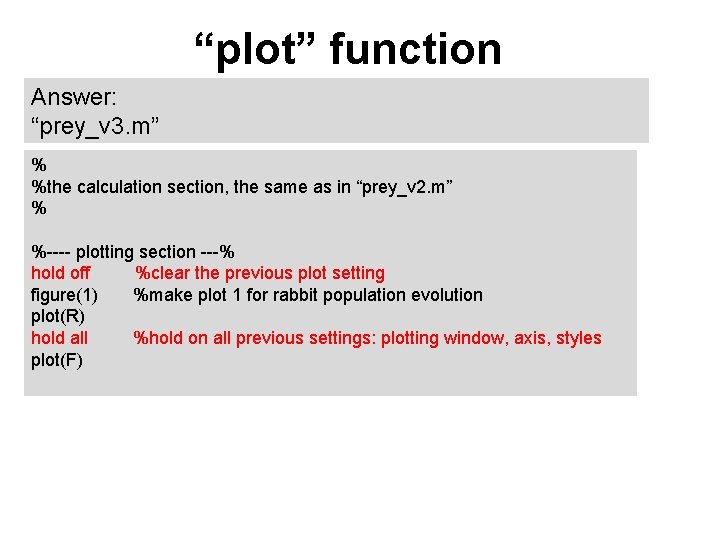
“plot” function Answer: “prey_v 3. m” % %the calculation section, the same as in “prey_v 2. m” % %---- plotting section ---% hold off %clear the previous plot setting figure(1) %make plot 1 for rabbit population evolution plot(R) hold all %hold on all previous settings: plotting window, axis, styles plot(F)

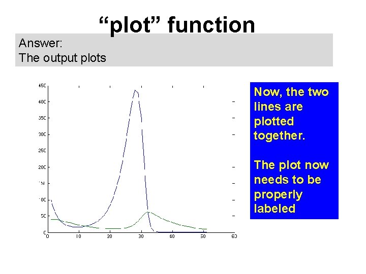
“plot” function Answer: The output plots Now, the two lines are plotted together. The plot now needs to be properly labeled

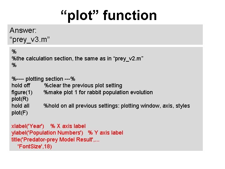
“plot” function Answer: “prey_v 3. m” % %the calculation section, the same as in “prey_v 2. m” % %---- plotting section ---% hold off %clear the previous plot setting figure(1) %make plot 1 for rabbit population evolution plot(R) hold all %hold on all previous settings: plotting window, axis, styles plot(F) xlabel('Year') % X axis label ylabel('Population Numbers') % Y axis label title('Predator-prey Model Result', . . . 'Font. Size', 18)

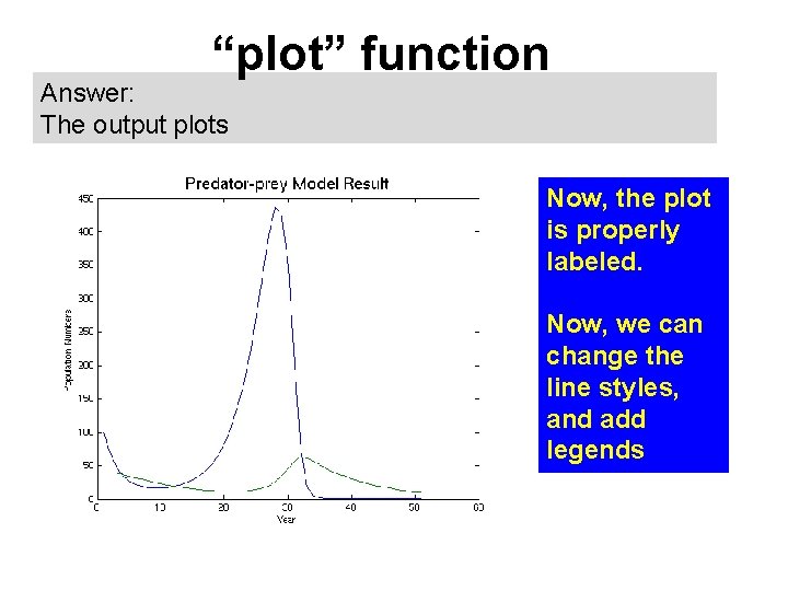
“plot” function Answer: The output plots Now, the plot is properly labeled. Now, we can change the line styles, and add legends

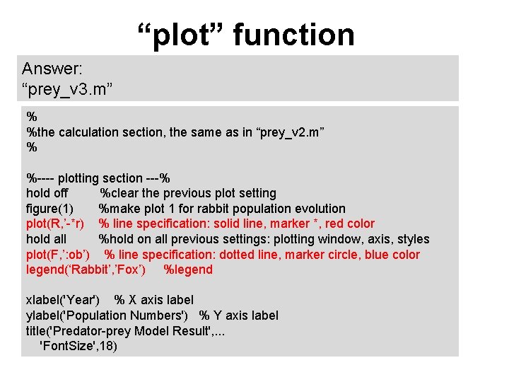
“plot” function Answer: “prey_v 3. m” % %the calculation section, the same as in “prey_v 2. m” % %---- plotting section ---% hold off %clear the previous plot setting figure(1) %make plot 1 for rabbit population evolution plot(R, ’-*r) % line specification: solid line, marker *, red color hold all %hold on all previous settings: plotting window, axis, styles plot(F, ’: ob’) % line specification: dotted line, marker circle, blue color legend(‘Rabbit’, ’Fox’) %legend xlabel('Year') % X axis label ylabel('Population Numbers') % Y axis label title('Predator-prey Model Result', . . . 'Font. Size', 18)

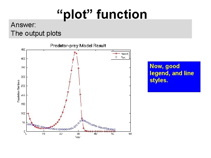
“plot” function Answer: The output plots Now, good legend, and line styles.

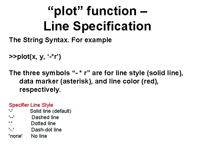
“plot” function – Line Specification The String Syntax. For example >>plot(x, y, ‘-*r’) The three symbols “- * r” are for line style (solid line), data marker (asterisk), and line color (red), respectively. Specifier Line Style '-' Solid line (default) '--' Dashed line ': ' Dotted line '-. ' Dash-dot line 'none' No line

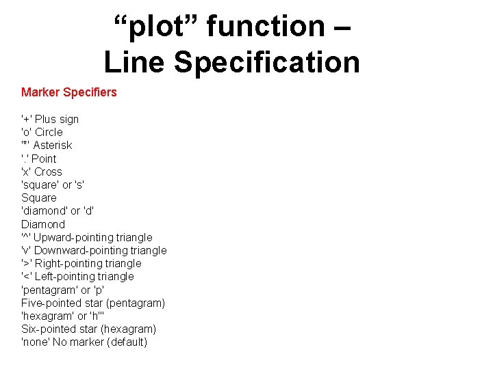
“plot” function – Line Specification Marker Specifiers '+' Plus sign 'o' Circle '*' Asterisk '. ' Point 'x' Cross 'square' or 's' Square 'diamond' or 'd' Diamond '^' Upward-pointing triangle 'v' Downward-pointing triangle '>' Right-pointing triangle '<' Left-pointing triangle 'pentagram' or 'p' Five-pointed star (pentagram) 'hexagram' or 'h''' Six-pointed star (hexagram) 'none' No marker (default)

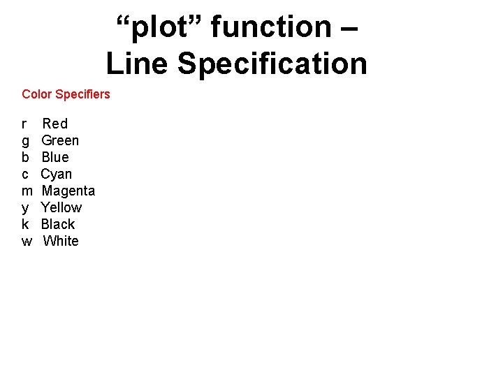
“plot” function – Line Specification Color Specifiers r g b c m y k w Red Green Blue Cyan Magenta Yellow Black White

“plot” function “Interaction plotting” Click on the right-most button on the Figure window, it will lead you to the interactive plotting tool. It is powerful. The learning of this tool is optional. Watch the video: http: //www. mathworks. com/products/featured/videos/? vid eo=Interactively-Creating-Plots

“plot” function Find more information about “plot” or any other build-in functions, you can click on the question “? ” mark on the main Matlab window, then type “plot” in the search window.

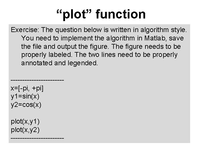
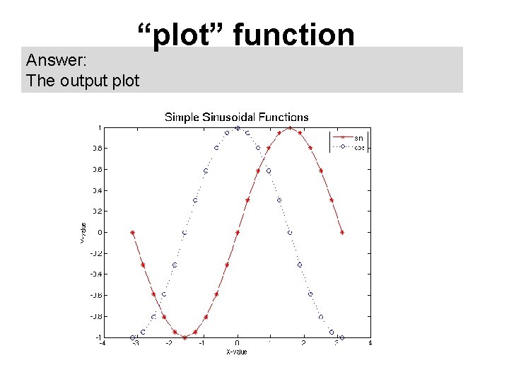
“plot” function Exercise: The question below is written in algorithm style. You need to implement the algorithm in Matlab, save the file and output the figure. The figure needs to be properly labeled. The two lines need to be properly annotated and legended. -----------x=[-pi, +pi] y 1=sin(x) y 2=cos(x) plot(x, y 1) plot(x, y 2) ------------

“plot” function Answer: “sin. m” clear %clear the variable %----model calculation section--x=[-pi: pi/10: pi] %create twenty data points y 1=sin(x) % y 2=cos(x) %---- plotting section ---% hold off %clear the previous plot setting figure(1) %make plot in figure 1 plot(x, y 1, '-*r') %line specification: solid line, marker *, red color hold all %hold on all previous settings: plotting window, axis, styles plot(x, y 2, ': ob') %line specification: dotted line, marker circle, blue legend('sin', 'cos') xlabel('X-value') % X axis label ylabel('Y-value') % Y axis label title('Simple Sinusoidal Functions', . . . 'Font. Size', 18)

“plot” function Answer: The output plot

(Oct. 06, 2011 Stops Here)

(Oct. 20, 2011 Starts Here)

SS-3 Computational Models SS-3. 1 – A Few Basics SS-3. 2 – Differentiation SS-3. 3 -- Integration

SS-3. 1 Computational Models – A Few Basics Objectives: 1. Algorithm 2. Iteration 3. Initial Condition 4. Interval and Sub-interval I have so far treated a computational model as programming and implementation, and have run many examples. Now, let me introduce a few formal concepts associated with a computational model

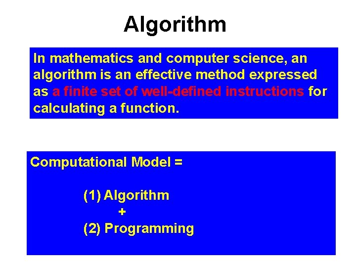
Algorithm In mathematics and computer science, an algorithm is an effective method expressed as a finite set of well-defined instructions for calculating a function. Computational Model = (1) Algorithm + (2) Programming

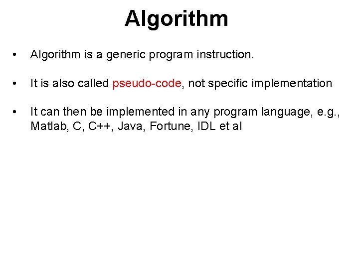
Algorithm • Algorithm is a generic program instruction. • It is also called pseudo-code, not specific implementation • It can then be implemented in any program language, e. g. , Matlab, C, C++, Java, Fortune, IDL et al

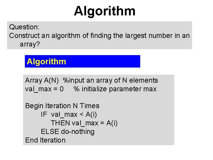
Algorithm Question: Construct an algorithm of finding the largest number in an array? Algorithm Array A(N) %input an array of N elements val_max = 0 % initialize parameter max Begin Iteration N Times IF val_max < A(i) THEN val_max = A(i) ELSE do-nothing End Iteration

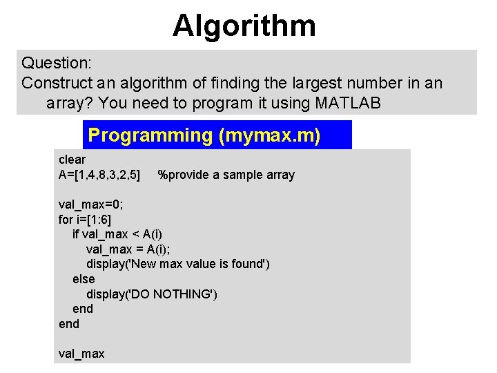
Algorithm Question: Construct an algorithm of finding the largest number in an array? You need to program it using MATLAB Programming (mymax. m) clear A=[1, 4, 8, 3, 2, 5] %provide a sample array val_max=0; for i=[1: 6] if val_max < A(i) val_max = A(i); display('New max value is found') else display('DO NOTHING') end val_max

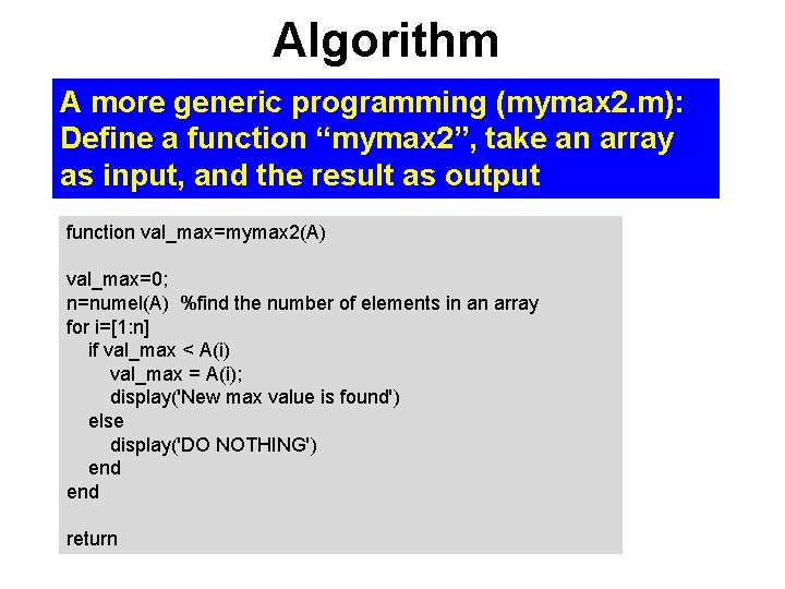
Algorithm A more generic programming (mymax 2. m): Define a function “mymax 2”, take an array as input, and the result as output function val_max=mymax 2(A) val_max=0; n=numel(A) %find the number of elements in an array for i=[1: n] if val_max < A(i) val_max = A(i); display('New max value is found') else display('DO NOTHING') end return

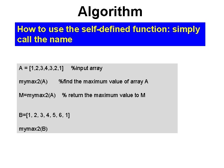
Algorithm How to use the self-defined function: simply call the name A = [1, 2, 3, 4, 3, 2, 1] mymax 2(A) M=mymax 2(A) %find the maximum value of array A % return the maximum value to M B=[1, 2, 3, 4, 5, 6, 1] mymax 2(B) %input array

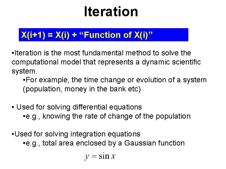
Iteration X(i+1) = X(i) + “Function of X(i)” • Iteration is the most fundamental method to solve the computational model that represents a dynamic scientific system. • For example, the time change or evolution of a system (population, money in the bank etc) • Used for solving differential equations • e. g. , knowing the rate of change of the population • Used for solving integration equations • e. g. , total area enclosed by a Gaussian function

Iteration >for i=[1: N] >X(i+1) = X(i) + “FUNCTION of X(i)”; >end • The output of current iteration is used as the input of the next iteration i: the sequence number of the iteration, representing the independent variable, usually the “time”, e. g. , year in population growth N: total number of iterations X: the dependent variable, an unknown function, but the model seeks to find FUNCTION(X(i)): the known function representing the knwwledge or model of the system

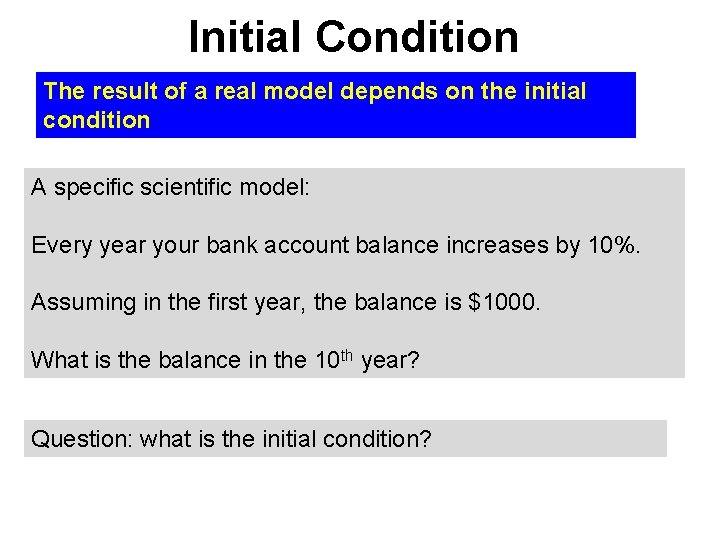
Initial Condition The result of a real model depends on the initial condition A specific scientific model: Every year your bank account balance increases by 10%. Assuming in the first year, the balance is $1000. What is the balance in the 10 th year? Question: what is the initial condition?

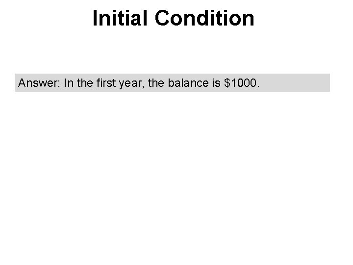
Initial Condition Answer: In the first year, the balance is $1000.

Interval and Sub-Interval The result of a real model depends on the interval and sub-interval. A specific scientific model: Every year your bank account balance increases by 12%. Assuming in the first year, the balance is $1000. What is the balance in the 10 th year? Question: what is the interval of the model? What is the sub-interval of the model?

Interval and Sub-Interval Answer: The interval is from year 1 to year 10. The sub-interval is every one year. Question: what will happen if the sub-interval changes? Does it change the result?

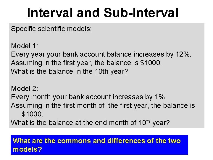
Interval and Sub-Interval Specific scientific models: Model 1: Every year your bank account balance increases by 12%. Assuming in the first year, the balance is $1000. What is the balance in the 10 th year? Model 2: Every month your bank account increases by 1% Assuming in the first month of the first year, the balance is $1000. What is the balance at the end month of 10 th year? What are the commons and differences of the two models?

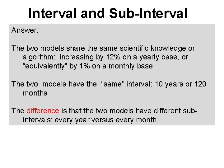
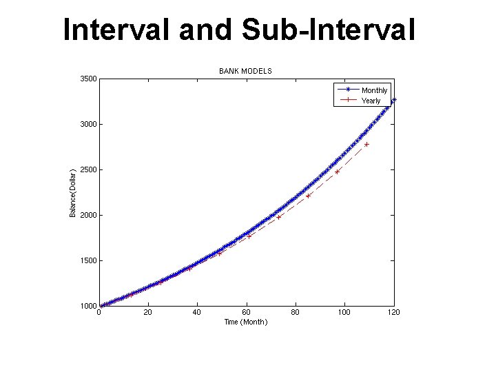
Interval and Sub-Interval Answer: The two models share the same scientific knowledge or algorithm: increasing by 12% on a yearly base, or “equivalently” by 1% on a monthly base The two models have the “same” interval: 10 years or 120 months The difference is that the two models have different subintervals: every year versus every month

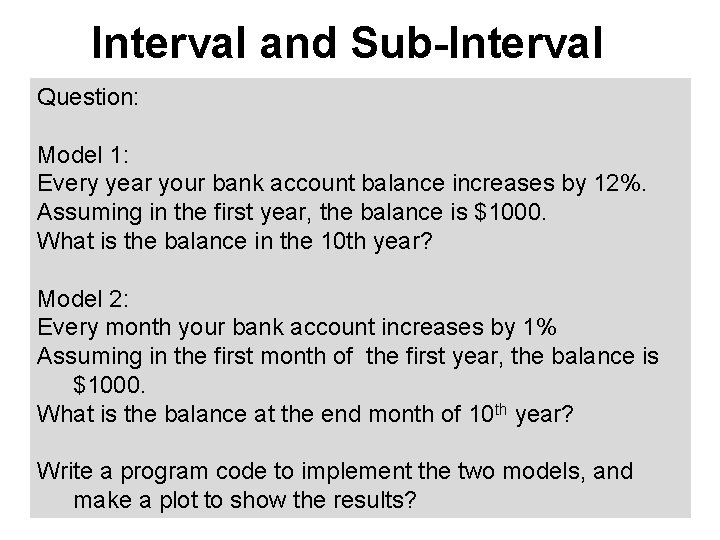
Interval and Sub-Interval Question: Model 1: Every year your bank account balance increases by 12%. Assuming in the first year, the balance is $1000. What is the balance in the 10 th year? Model 2: Every month your bank account increases by 1% Assuming in the first month of the first year, the balance is $1000. What is the balance at the end month of 10 th year? Write a program code to implement the two models, and make a plot to show the results?

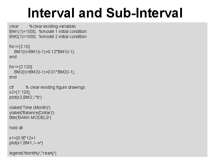
Interval and Sub-Interval clear %clear existing variables BM 1(1)=1000; %model 1 initial condition BM 2(1)=1000; %model 2 initial condition for i=[2: 10] BM 1(i)=BM 1(i-1)+0. 12*BM 1(i-1); end for i=[2: 120] BM 2(i)=BM 2(i-1)+0. 01*BM 2(i-1); end clf % clear existing figure drawings x 2=[1: 120]; plot(x 2, BM 2, '-*b') xlabel('Time (Month)') ylabel('Balance(Dollar)') title('BANK MODELS') hold all x 1=[0: 9]*12+1 plot(x 1, BM 1, '--+r') legend('Monthly', 'Yearly')

Interval and Sub-Interval

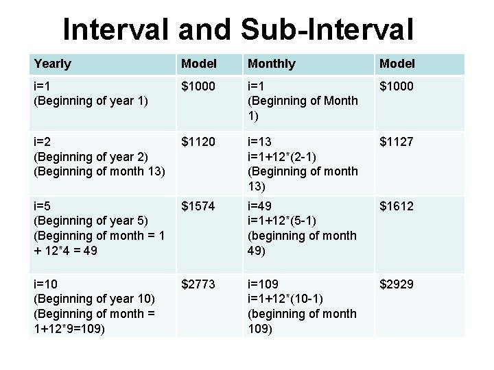
Interval and Sub-Interval Yearly Model Monthly Model i=1 (Beginning of year 1) $1000 i=1 (Beginning of Month 1) $1000 i=2 (Beginning of year 2) (Beginning of month 13) $1120 i=13 i=1+12*(2 -1) (Beginning of month 13) $1127 i=5 (Beginning of year 5) (Beginning of month = 1 + 12*4 = 49 $1574 i=49 i=1+12*(5 -1) (beginning of month 49) $1612 i=10 (Beginning of year 10) (Beginning of month = 1+12*9=109) $2773 i=109 i=1+12*(10 -1) (beginning of month 109) $2929

Interval and Sub-interval • In numerical simulation, one has to specify the calculation interval and sub-interval • Interval is the domain of the calculation • Sub-interval is the step-size in each iteration of the numerical calculation • We have assumed that the sub-interval is every one year in many examples. But this is for convenience only, it can be every one month.

The Effects of Sub-interval • A smaller sub-interval requires more steps of calculation • But, a smaller sub-interval provides more detailed evolution • Further, a smaller sub-interval provides a more accurate result • This point will be further illustrated in the context of differentiation and integration

(Oct. 20, 2011 Stops Here)

(Oct. 25, 2011 Starts Here)

SS-3. 2: Computational Model -- Differentiation (Oct. 25, 2011)

Review • Algorithm • Iteration • Initial Condition • Interval • Sub-interval

Review: Interval and Sub-interval • In numerical simulation, one has to specify the calculation interval and sub-interval • Interval is the domain of the calculation • Sub-interval is the step-size in each iteration of the numerical calculation • We have assumed that the sub-interval is every one year in many examples. But this is for convenience only. The sub-interval can be every one month, or even shorter.

Review: The Effects of Sub-interval • A smaller sub-interval requires more steps of calculation • But, a smaller sub-interval provides more detailed evolution • Further, a smaller sub-interval provides a more accurate result. • One branch of computational science is to find the balance between computational cost and the accuracy: minimize the number of calculations, and maximum the accuracy.

Differential Equations Differential equations play an important role in modeling virtually every physical, technical, or biological process, from celestial motion, to bridge design, to interactions between neurons (http: //en. wikipedia. org/wiki/Differential_equation)

Differential Equations • It is an equation to describe the rate of change of one parameter (or several parameters) in a scientific system • The rate of change could be in time (t) • The rate of change could also be in position, along x in one dimension, along (x, y) in two dimensions, and along (x, y, z) in three dimensions

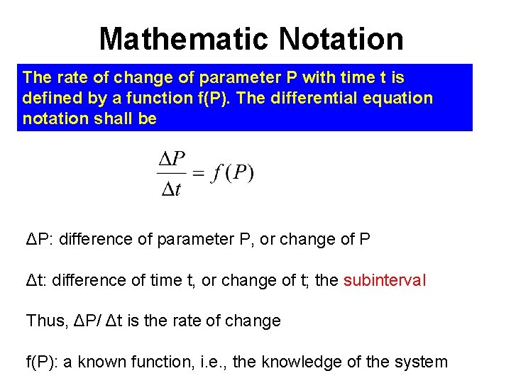
Mathematic Notation The rate of change of parameter P with time t is defined by a function f(P). The differential equation notation shall be ΔP: difference of parameter P, or change of P Δt: difference of time t, or change of t; the subinterval Thus, ΔP/ Δt is the rate of change f(P): a known function, i. e. , the knowledge of the system

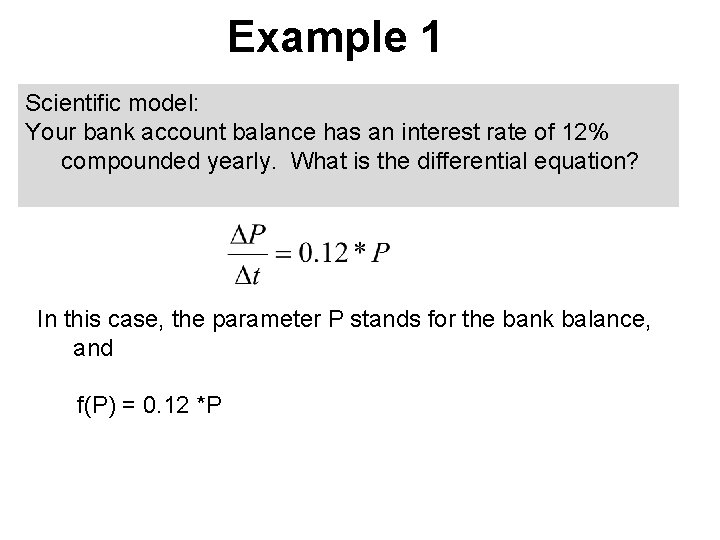
Example 1 Scientific model: Your bank account balance has an interest rate of 12% compounded yearly. What is the differential equation? In this case, the parameter P stands for the bank balance, and f(P) = 0. 12 *P

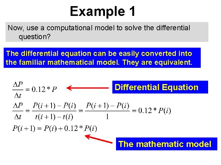
Example 1 Now, use a computational model to solve the differential question? The differential equation can be easily converted into the familiar mathematical model. They are equivalent. Differential Equation The mathematic model

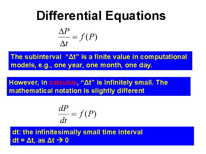
Differential Equations The subinterval “Δt” is a finite value in computational models, e. g. , one year, one month, one day. However, in calculus, “Δt” is infinitely small. The mathematical notation is slightly different dt: the infinitesimally small time interval dt = Δt, as Δt 0

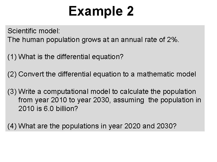
Example 2 Scientific model: The human population grows at an annual rate of 2%. (1) What is the differential equation? (2) Convert the differential equation to a mathematic model (3) Write a computational model to calculate the population from year 2010 to year 2030, assuming the population in 2010 is 6. 0 billion? (4) What are the populations in year 2020 and 2030?

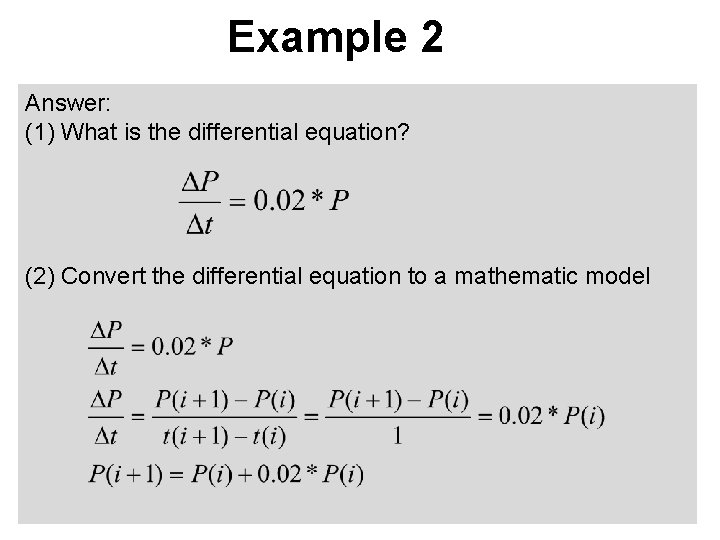
Example 2 Answer: (1) What is the differential equation? (2) Convert the differential equation to a mathematic model

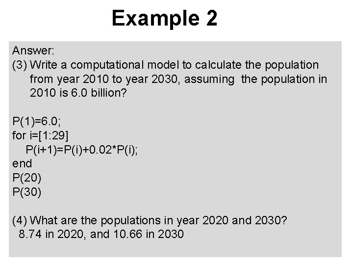
Example 2 Answer: (3) Write a computational model to calculate the population from year 2010 to year 2030, assuming the population in 2010 is 6. 0 billion? P(1)=6. 0; for i=[1: 29] P(i+1)=P(i)+0. 02*P(i); end P(20) P(30) (4) What are the populations in year 2020 and 2030? 8. 74 in 2020, and 10. 66 in 2030

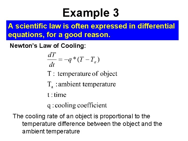
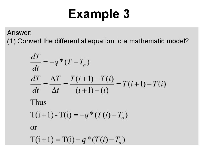
Example 3 A scientific law is often expressed in differential equations, for a good reason. Newton’s Law of Cooling: The cooling rate of an object is proportional to the temperature difference between the object and the ambient temperature

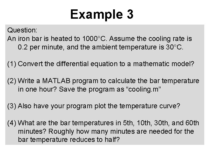
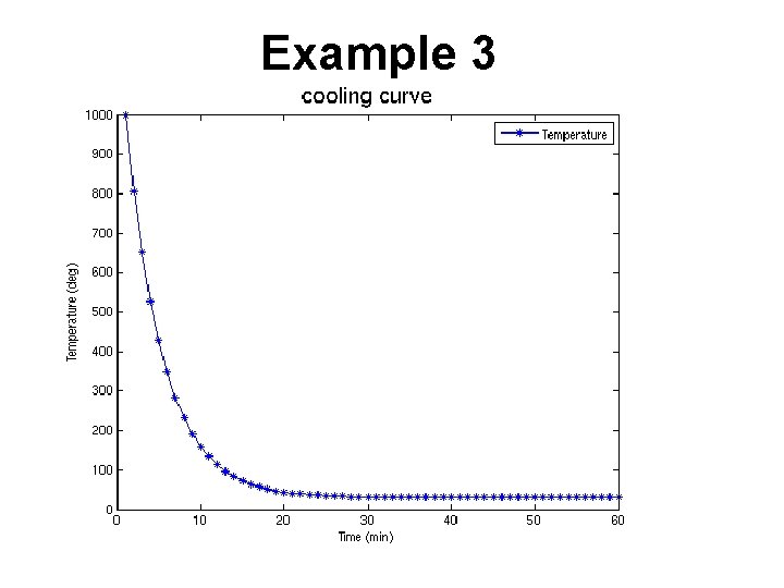
Example 3 Question: An iron bar is heated to 1000°C. Assume the cooling rate is 0. 2 per minute, and the ambient temperature is 30°C. (1) Convert the differential equation to a mathematic model? (2) Write a MATLAB program to calculate the bar temperature in one hour? Save the program as “cooling. m” (3) Also have your program plot the temperature curve? (4) What are the bar temperatures in 5 th, 10 th, 30 th, and 60 th minutes? Roughly how many minutes are needed for the bar temperature reduces to half?

Example 3 Answer: (1) Convert the differential equation to a mathematic model?

“cooling. m” function [T] = cooling () clear T(1)=1000 % initial temperature Ta=30 % ambient temperature q = 0. 2 % cooling coefficient N=60 % interval 60 minutes for i=[1: N-1] T(i+1)=T(i)-q*(T(i)-Ta); end plot(T, '-*b') xlabel('Time (min)') ylabel('Temperature (deg)') title('cooling curve', 'Font. Size', 18) legend('Temperature') sprintf('Temperature in 5 th minute = %f', T(5)) %create a string to be displayed sprintf('Temperature in 10 th minute = %f', T(10)) sprintf('Temperature in 30 th minute = %f', T(30)) sprintf('Temperature in 60 th minute = %f', T(60)) end

Example 3

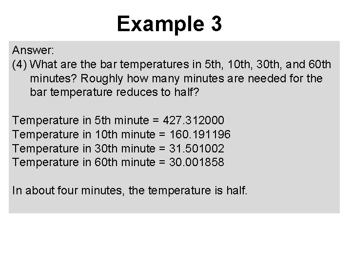
Example 3 Answer: (4) What are the bar temperatures in 5 th, 10 th, 30 th, and 60 th minutes? Roughly how many minutes are needed for the bar temperature reduces to half? Temperature in 5 th minute = 427. 312000 Temperature in 10 th minute = 160. 191196 Temperature in 30 th minute = 31. 501002 Temperature in 60 th minute = 30. 001858 In about four minutes, the temperature is half.

(Oct. 25, 2011 Stops Here)

(Oct. 27, 2011 Starts Here)

SS-3. 3: Computational Model -- Integration (Oct. 27, 2011)

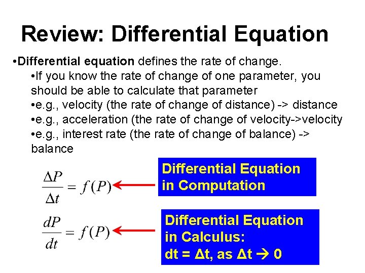
Review: Differential Equation • Differential equation defines the rate of change. • If you know the rate of change of one parameter, you should be able to calculate that parameter • e. g. , velocity (the rate of change of distance) -> distance • e. g. , acceleration (the rate of change of velocity->velocity • e. g. , interest rate (the rate of change of balance) -> balance Differential Equation in Computation Differential Equation in Calculus: dt = Δt, as Δt 0

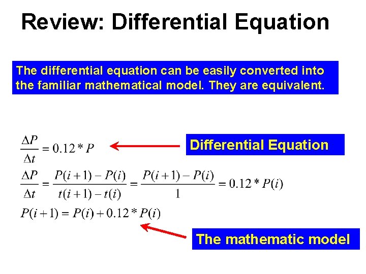
Review: Differential Equation The differential equation can be easily converted into the familiar mathematical model. They are equivalent. Differential Equation The mathematic model

Integration • Integration is to find the sum of a function. • It is related to differentiation. It is just exactly the opposite operation of a differentiation. Both integration and differentiation address the same scientific question • e. g. , known the velocity, find the distance • The relation is similar to that of between division (differentiation) and multiplication (integration)

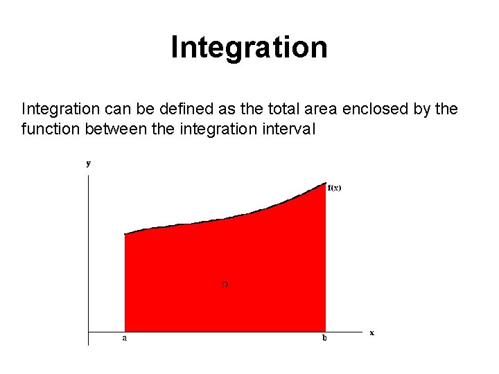
Integration can be defined as the total area enclosed by the function between the integration interval

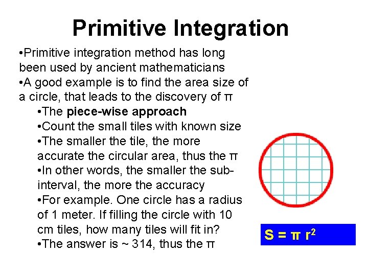
Primitive Integration • Primitive integration method has long been used by ancient mathematicians • A good example is to find the area size of a circle, that leads to the discovery of π • The piece-wise approach • Count the small tiles with known size • The smaller the tile, the more accurate the circular area, thus the π • In other words, the smaller the subinterval, the more the accuracy • For example. One circle has a radius of 1 meter. If filling the circle with 10 cm tiles, how many tiles will fit in? • The answer is ~ 314, thus the π S = π r 2

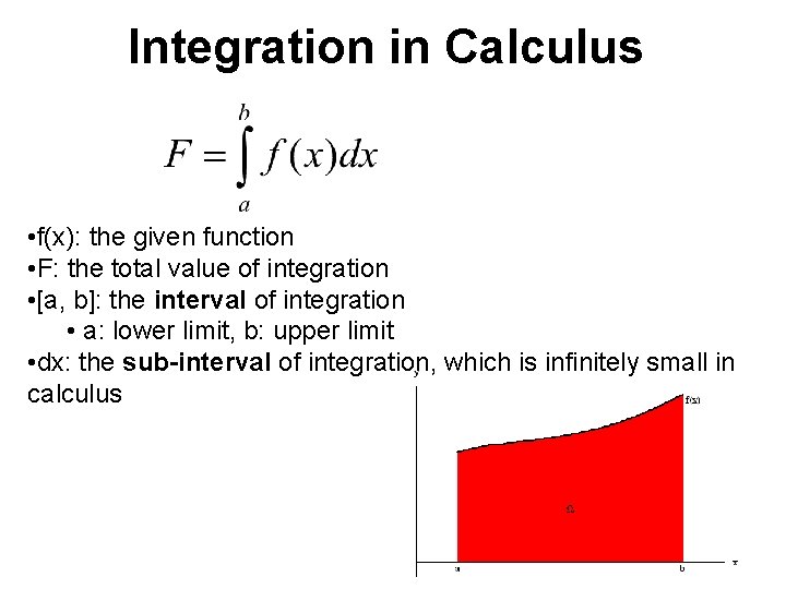
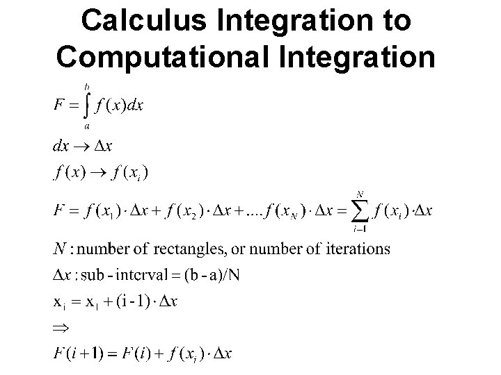
Integration in Calculus • f(x): the given function • F: the total value of integration • [a, b]: the interval of integration • a: lower limit, b: upper limit • dx: the sub-interval of integration, which is infinitely small in calculus

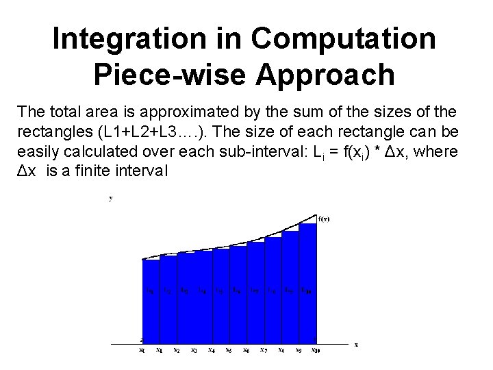
Integration in Computation Piece-wise Approach The total area is approximated by the sum of the sizes of the rectangles (L 1+L 2+L 3…. ). The size of each rectangle can be easily calculated over each sub-interval: Li = f(xi) * Δx, where Δx is a finite interval

Calculus Integration to Computational Integration

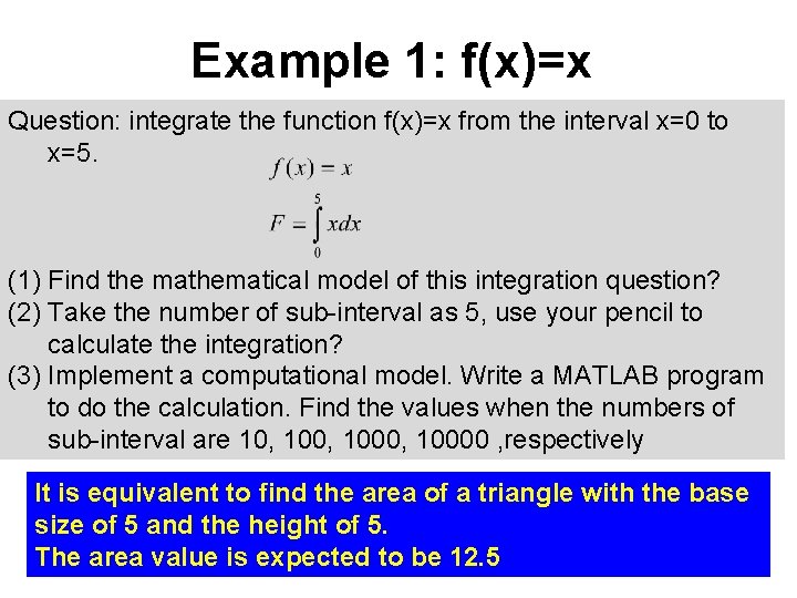
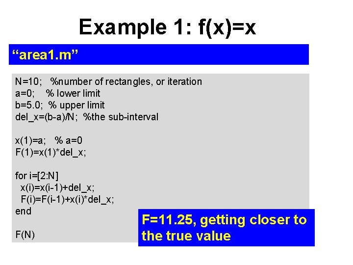
Example 1: f(x)=x Question: integrate the function f(x)=x from the interval x=0 to x=5. (1) Find the mathematical model of this integration question? (2) Take the number of sub-interval as 5, use your pencil to calculate the integration? (3) Implement a computational model. Write a MATLAB program to do the calculation. Find the values when the numbers of sub-interval are 10, 1000, 10000 , respectively It is equivalent to find the area of a triangle with the base size of 5 and the height of 5. The area value is expected to be 12. 5

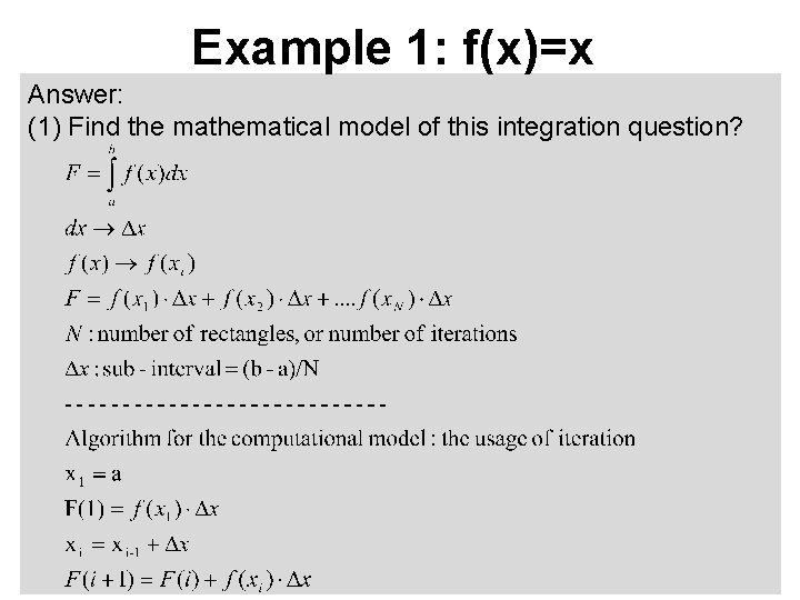
Example 1: f(x)=x Answer: (1) Find the mathematical model of this integration question?

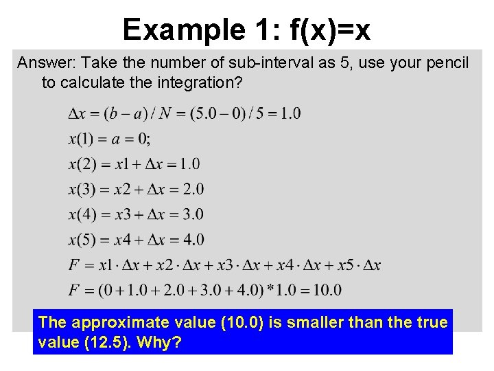
Example 1: f(x)=x Answer: Take the number of sub-interval as 5, use your pencil to calculate the integration? The approximate value (10. 0) is smaller than the true value (12. 5). Why?

Example 1: f(x)=x “area 1. m” N=10; %number of rectangles, or iteration a=0; % lower limit b=5. 0; % upper limit del_x=(b-a)/N; %the sub-interval x(1)=a; % a=0 F(1)=x(1)*del_x; for i=[2: N] x(i)=x(i-1)+del_x; F(i)=F(i-1)+x(i)*del_x; end F(N) F=11. 25, getting closer to the true value

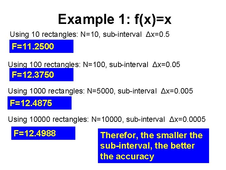
Example 1: f(x)=x Using 10 rectangles: N=10, sub-interval Δx=0. 5 F=11. 2500 Using 100 rectangles: N=100, sub-interval Δx=0. 05 F=12. 3750 Using 1000 rectangles: N=5000, sub-interval Δx=0. 005 F=12. 4875 Using 10000 rectangles: N=10000, sub-interval Δx=0. 0005 F=12. 4988 Therefor, the smaller the sub-interval, the better the accuracy

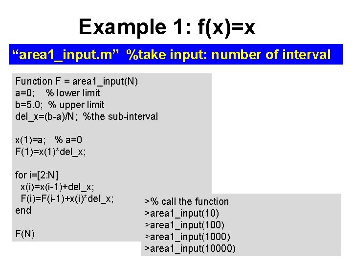
Example 1: f(x)=x “area 1_input. m” %take input: number of interval Function F = area 1_input(N) a=0; % lower limit b=5. 0; % upper limit del_x=(b-a)/N; %the sub-interval x(1)=a; % a=0 F(1)=x(1)*del_x; for i=[2: N] x(i)=x(i-1)+del_x; F(i)=F(i-1)+x(i)*del_x; end F(N) >% call the function >area 1_input(10) >area 1_input(1000) >area 1_input(10000)

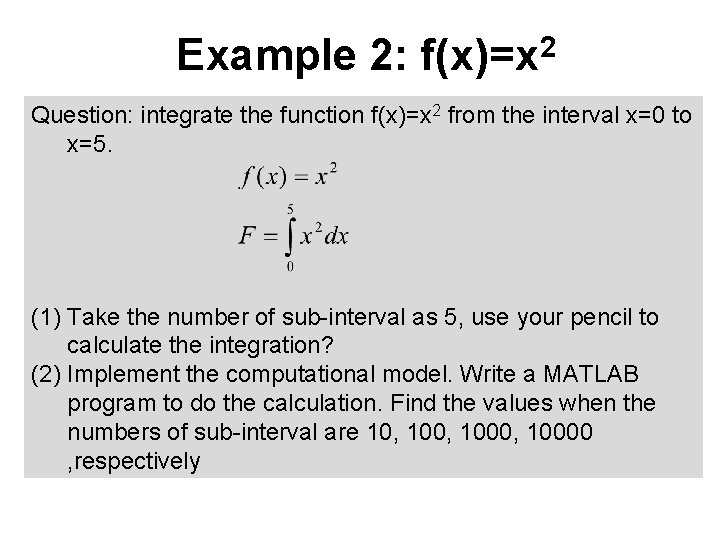
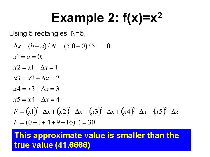
Example 2: f(x)=x 2 Question: integrate the function f(x)=x 2 from the interval x=0 to x=5. (1) Take the number of sub-interval as 5, use your pencil to calculate the integration? (2) Implement the computational model. Write a MATLAB program to do the calculation. Find the values when the numbers of sub-interval are 10, 1000, 10000 , respectively

Example 2: 2 f(x)=x Using 5 rectangles: N=5, This approximate value is smaller than the true value (41. 6666)

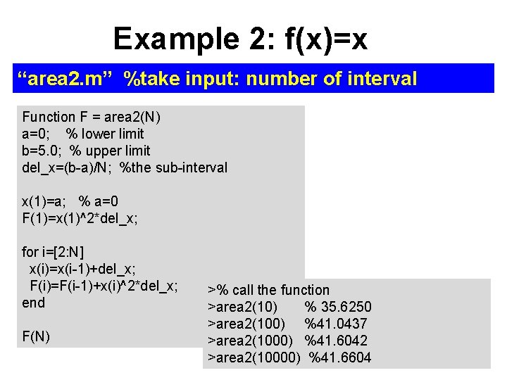
Example 2: f(x)=x “area 2. m” %take input: number of interval Function F = area 2(N) a=0; % lower limit b=5. 0; % upper limit del_x=(b-a)/N; %the sub-interval x(1)=a; % a=0 F(1)=x(1)^2*del_x; for i=[2: N] x(i)=x(i-1)+del_x; F(i)=F(i-1)+x(i)^2*del_x; end F(N) >% call the function >area 2(10) % 35. 6250 >area 2(100) %41. 0437 >area 2(1000) %41. 6042 >area 2(10000) %41. 6604

SS-4: Scientific Method (Oct. 27, 2011)

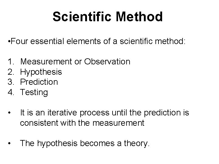
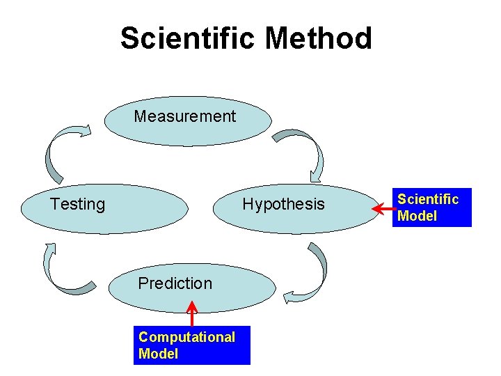
Scientific Method • Four essential elements of a scientific method: 1. 2. 3. 4. Measurement or Observation Hypothesis Prediction Testing • It is an iterative process until the prediction is consistent with the measurement • The hypothesis becomes a theory.

Scientific Method Measurement Testing Hypothesis Prediction Computational Model Scientific Model

The end