Scientific Computing a tutorial Sergey Pankratov Sergey Pankratov

Scientific Computing (a tutorial) Sergey Pankratov © Sergey Pankratov, 2002 1

Chapter 1. Mathematical Methods with Maple • Computer algebra systems in scientific computing (see e. g. J. Gathen, J. Gerhard. Modern Computer Algebra. Cambridge University Press, 1999; M. J. Wester. Computer Algebra Systems: A Practical Guide, John Wiley, 1999) • Maple – an interactive system, allowing one to carry out both numerical and analytical computations. Maple contains 2 D and 3 D graphical means, powerful programming language and an extensive library of mathematical formulae • A convenient working method, when all stages of mathematical, physical or engineering research can be stored in a single document - worksheet • The worksheet automatically becomes a scientific article, report, chapter in a book, etc. Chapter 1. Mathematical Methods with Maple Scientific Computing (a tutorial), Sergey Pankratov, 2002 2

Literature on Maple • A. Heck, Introduction to Maple. Springer, 1996 • M. B. Monagan, K. O. Geddes, K. M. Heal, G. Labahn, S. M. Vorkoetter, J. Mc. Carron. Maple 6. Programming Guide. Waterloo Maple Inc. 2000 • K. M. Heal, M. L. Hansen, K. M. Rickard. Maple 6. Learning Guide. Waterloo Maple Inc. 2000 • D. Redfern. The Maple Handbook. Springer, 1996 • W. Gandler, J. Hrebicek. Solving Problems in Scientific Computing Using Maple and MATLAB. Springer, 1995 • E. Kamerich. A Guide to Maple. Springer, 1999 Chapter 1. Mathematical Methods with Maple Scientific Computing (a tutorial), Sergey Pankratov, 2002 3

Contents overview of the Chapter 1 General: • Maple has an extensive Help facility, it is an essential aid Chapter 1. Mathematical Methods with Maple Scientific Computing (a tutorial), Sergey Pankratov, 2002 4

Document organization in Maple • One should familiarize oneself with Maple GUI • The best way is to learn use and syntax of Maple simultaneously and by examples • A worksheet (*. mws) consists of logical groups called „execution groups“ Each group consists of several parts : - Input Region - Output Region - Text Region (e. g. comments) • The principal objects in Maple: numbers, constants, names - numbers: integer, real, rational, radicals - constants: Pi, I, E, Infinity, gamma, true, false - names: sequences of symbols starting with literal (e. g. new, New, new_old, etc. ) Chapter 1. Mathematical Methods with Maple Scientific Computing (a tutorial), Sergey Pankratov, 2002 5

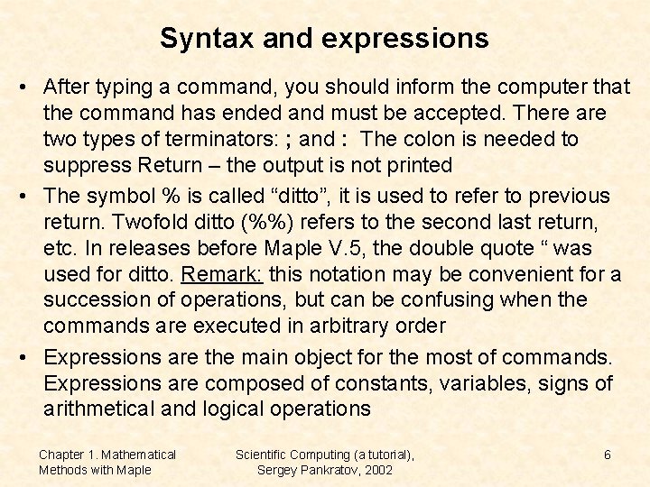
Syntax and expressions • After typing a command, you should inform the computer that the command has ended and must be accepted. There are two types of terminators: ; and : The colon is needed to suppress Return – the output is not printed • The symbol % is called “ditto”, it is used to refer to previous return. Twofold ditto (%%) refers to the second last return, etc. In releases before Maple V. 5, the double quote “ was used for ditto. Remark: this notation may be convenient for a succession of operations, but can be confusing when the commands are executed in arbitrary order • Expressions are the main object for the most of commands. Expressions are composed of constants, variables, signs of arithmetical and logical operations Chapter 1. Mathematical Methods with Maple Scientific Computing (a tutorial), Sergey Pankratov, 2002 6

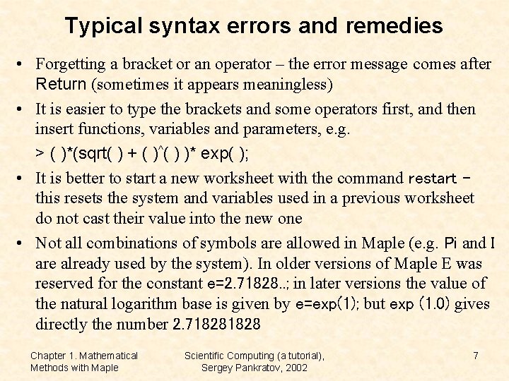
Typical syntax errors and remedies • Forgetting a bracket or an operator – the error message comes after Return (sometimes it appears meaningless) • It is easier to type the brackets and some operators first, and then insert functions, variables and parameters, e. g. > ( )*(sqrt( ) + ( )^( ) )* exp( ); • It is better to start a new worksheet with the command restart – this resets the system and variables used in a previous worksheet do not cast their value into the new one • Not all combinations of symbols are allowed in Maple (e. g. Pi and I are already used by the system). In older versions of Maple E was reserved for the constant e=2. 71828. . ; in later versions the value of the natural logarithm base is given by e=exp(1); but exp (1. 0) gives directly the number 2. 71828 Chapter 1. Mathematical Methods with Maple Scientific Computing (a tutorial), Sergey Pankratov, 2002 7

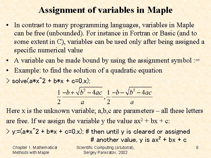
Assignment of variables in Maple • In contrast to many programming languages, variables in Maple can be free (unbounded). For instance in Fortran or Basic (and to some extent in C), variables can be used only after being assigned a specific numerical value • A variable can be made bound by using the assignment symbol : = • Example: to find the solution of a quadratic equation > solve(a*x^2 + b*x + c=0, x); Here x is the unknown variable; a, b, c are parameters – all these letters are free. If we assign the variable y the value ax 2 + bx + c: > y: =(a*x^2 + b*x + c=0, x); # then until y is cleared or assigned # another value, y is ax 2 + bx + c Chapter 1. Mathematical Methods with Maple Scientific Computing (a tutorial), Sergey Pankratov, 2002 8

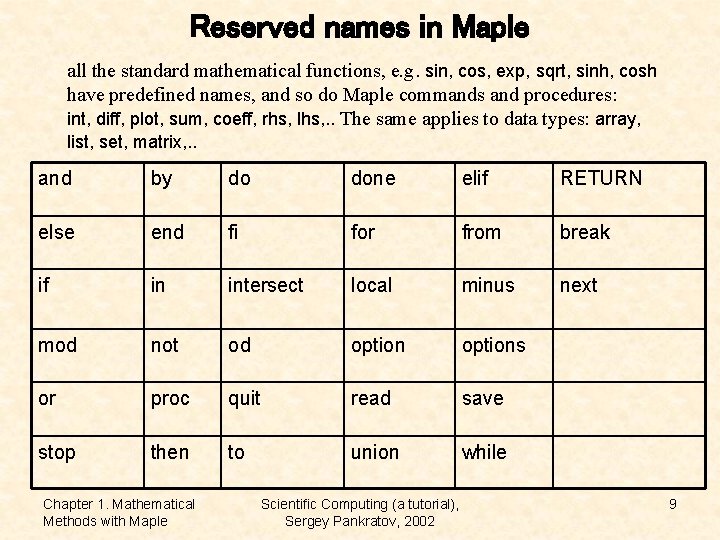
Reserved names in Maple all the standard mathematical functions, e. g. sin, cos, exp, sqrt, sinh, cosh have predefined names, and so do Maple commands and procedures: int, diff, plot, sum, coeff, rhs, lhs, . . The same applies to data types: array, list, set, matrix, . . and by do done elif RETURN else end fi for from break if in intersect local minus next mod not od options or proc quit read save stop then to union while Chapter 1. Mathematical Methods with Maple Scientific Computing (a tutorial), Sergey Pankratov, 2002 9

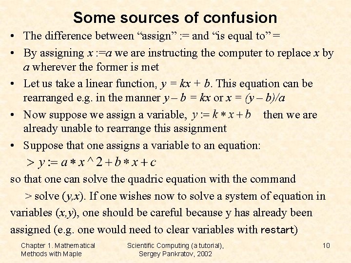
Some sources of confusion • The difference between “assign” : = and “is equal to” = • By assigning x : =a we are instructing the computer to replace x by a wherever the former is met • Let us take a linear function, y = kx + b. This equation can be rearranged e. g. in the manner y – b = kx or x = (y – b)/a • Now suppose we assign a variable, then we are already unable to rearrange this assignment • Suppose that one assigns a variable to an equation: so that one can solve the quadric equation with the command > solve (y, x). If one wishes now to solve a system of equation in variables (x, y), one should be careful because y has already been assigned (e. g. one would need to clear variables with restart) Chapter 1. Mathematical Methods with Maple Scientific Computing (a tutorial), Sergey Pankratov, 2002 10

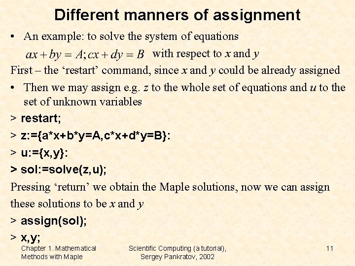
Different manners of assignment • An example: to solve the system of equations with respect to x and y First – the ‘restart’ command, since x and y could be already assigned • Then we may assign e. g. z to the whole set of equations and u to the set of unknown variables > restart; > z: ={a*x+b*y=A, c*x+d*y=B}: > u: ={x, y}: > sol: =solve(z, u); Pressing ‘return’ we obtain the Maple solutions, now we can assign these solutions to be x and y > assign(sol); > x, y; Chapter 1. Mathematical Methods with Maple Scientific Computing (a tutorial), Sergey Pankratov, 2002 11

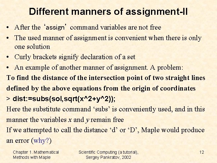
Different manners of assignment-II • After the ‘assign’ command variables are not free • The used manner of assignment is convenient when there is only one solution • Curly brackets signify declaration of a set • An example of another manner of assignment. A problem: To find the distance of the intersection point of two straight lines defined by the above equations from the origin of coordinates > dist: =subs(sol, sqrt(x^2+y^2)); Here the substitute command ‘subs’ is conveniently used, and in this manner the variables x and y remain free If we attempted to call the distance ‘d’ or ‘D’, Maple would produce an error (why? ) Chapter 1. Mathematical Methods with Maple Scientific Computing (a tutorial), Sergey Pankratov, 2002 12

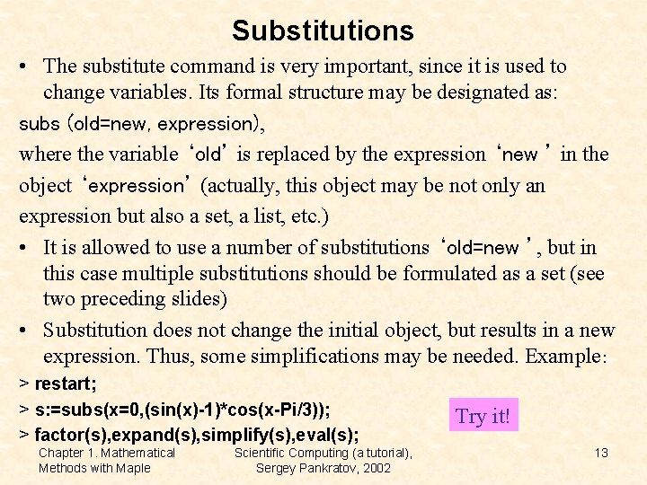
Substitutions • The substitute command is very important, since it is used to change variables. Its formal structure may be designated as: subs (old=new, expression), where the variable ‘old’ is replaced by the expression ‘new ’ in the object ‘expression’ (actually, this object may be not only an expression but also a set, a list, etc. ) • It is allowed to use a number of substitutions ‘old=new ’, but in this case multiple substitutions should be formulated as a set (see two preceding slides) • Substitution does not change the initial object, but results in a new expression. Thus, some simplifications may be needed. Example: > restart; > s: =subs(x=0, (sin(x)-1)*cos(x-Pi/3)); > factor(s), expand(s), simplify(s), eval(s); Chapter 1. Mathematical Methods with Maple Scientific Computing (a tutorial), Sergey Pankratov, 2002 Try it! 13

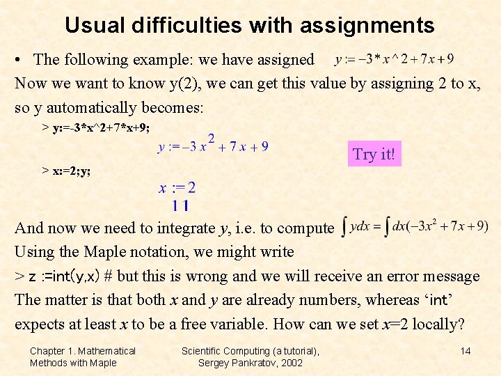
Usual difficulties with assignments • The following example: we have assigned Now we want to know y(2), we can get this value by assigning 2 to x, so y automatically becomes: > y: =-3*x^2+7*x+9; Try it! > x: =2; y; And now we need to integrate y, i. e. to compute Using the Maple notation, we might write > z : =int(y, x) # but this is wrong and we will receive an error message The matter is that both x and y are already numbers, whereas ‘int’ expects at least x to be a free variable. How can we set x=2 locally? Chapter 1. Mathematical Methods with Maple Scientific Computing (a tutorial), Sergey Pankratov, 2002 14

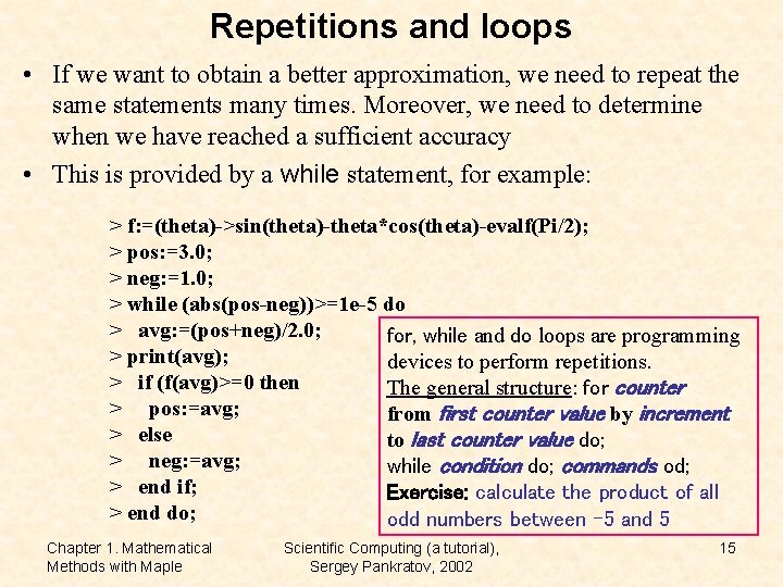
Repetitions and loops • If we want to obtain a better approximation, we need to repeat the same statements many times. Moreover, we need to determine when we have reached a sufficient accuracy • This is provided by a while statement, for example: > f: =(theta)->sin(theta)-theta*cos(theta)-evalf(Pi/2); > pos: =3. 0; > neg: =1. 0; > while (abs(pos-neg))>=1 e-5 do > avg: =(pos+neg)/2. 0; for, while and do loops are programming > print(avg); devices to perform repetitions. > if (f(avg)>=0 then The general structure: for counter > pos: =avg; from first counter value by increment > else to last counter value do; > neg: =avg; while condition do; commands od; > end if; Exercise: calculate the product of all > end do; odd numbers between -5 and 5 Chapter 1. Mathematical Methods with Maple Scientific Computing (a tutorial), Sergey Pankratov, 2002 15

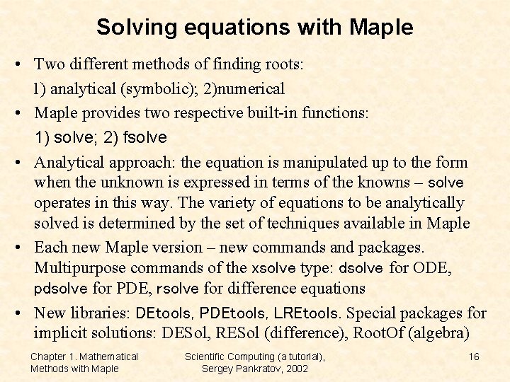
Solving equations with Maple • Two different methods of finding roots: 1) analytical (symbolic); 2)numerical • Maple provides two respective built-in functions: 1) solve; 2) fsolve • Analytical approach: the equation is manipulated up to the form when the unknown is expressed in terms of the knowns – solve operates in this way. The variety of equations to be analytically solved is determined by the set of techniques available in Maple • Each new Maple version – new commands and packages. Multipurpose commands of the xsolve type: dsolve for ODE, pdsolve for PDE, rsolve for difference equations • New libraries: DEtools, PDEtools, LREtools. Special packages for implicit solutions: DESol, RESol (difference), Root. Of (algebra) Chapter 1. Mathematical Methods with Maple Scientific Computing (a tutorial), Sergey Pankratov, 2002 16

Analytical solutions • The solve command – multipurpose, can be applied to systems of algebraic equations, inequalities, functional equations, identities. The form: solve (eqn, var), where eqn is an equation or a system of equations, var is a variable or a group of variables. If the latter parameter is absent, solve will look for solutions with respect to all symbolic variables • The system of equations and the group of variables are given as sets (in curly brackets and separated by commas) • Example: > s: =solve({6*x+y=sqrt(a), 3*x-2*y=4}, {x, y}); • If the equation is written without the equality sign it is viewed as one part of the equality, the other being considered zero: > sl: =solve(x^7+8*x, x); Chapter 1. Mathematical Methods with Maple Scientific Computing (a tutorial), Sergey Pankratov, 2002 17

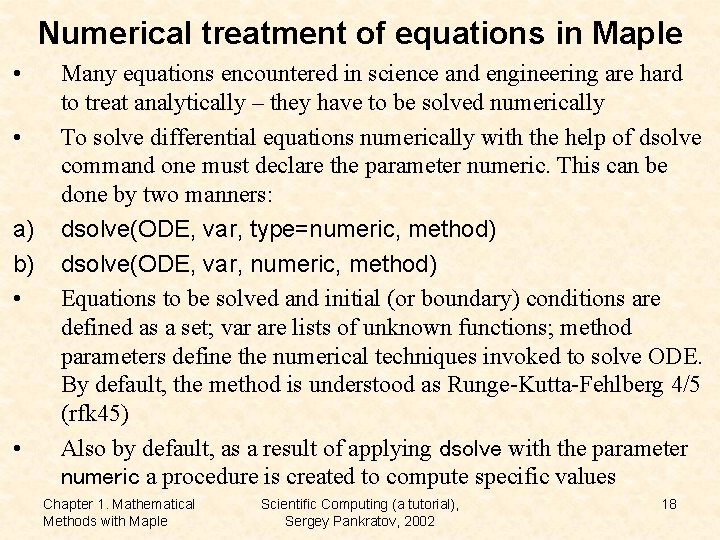
Numerical treatment of equations in Maple • • a) b) • • Many equations encountered in science and engineering are hard to treat analytically – they have to be solved numerically To solve differential equations numerically with the help of dsolve command one must declare the parameter numeric. This can be done by two manners: dsolve(ODE, var, type=numeric, method) dsolve(ODE, var, numeric, method) Equations to be solved and initial (or boundary) conditions are defined as a set; var are lists of unknown functions; method parameters define the numerical techniques invoked to solve ODE. By default, the method is understood as Runge-Kutta-Fehlberg 4/5 (rfk 45) Also by default, as a result of applying dsolve with the parameter numeric a procedure is created to compute specific values Chapter 1. Mathematical Methods with Maple Scientific Computing (a tutorial), Sergey Pankratov, 2002 18

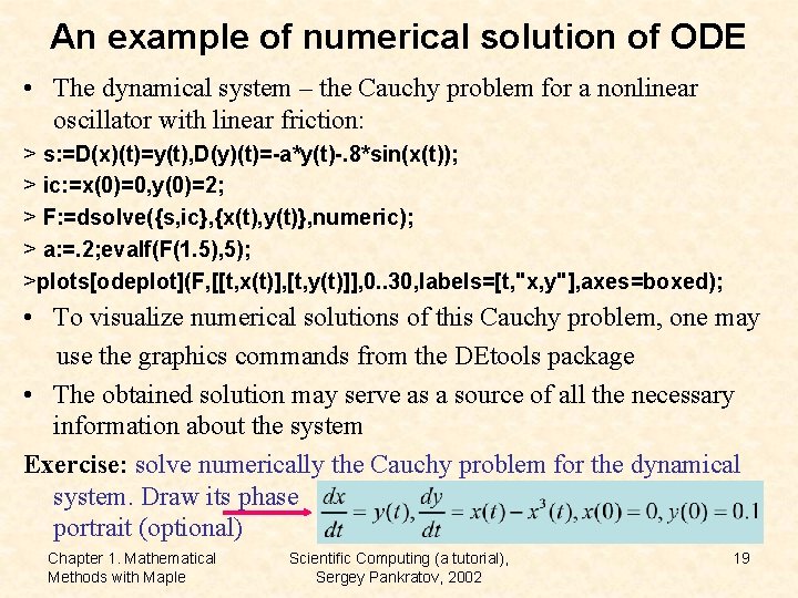
An example of numerical solution of ODE • The dynamical system – the Cauchy problem for a nonlinear oscillator with linear friction: > s: =D(x)(t)=y(t), D(y)(t)=-a*y(t)-. 8*sin(x(t)); > ic: =x(0)=0, y(0)=2; > F: =dsolve({s, ic}, {x(t), y(t)}, numeric); > a: =. 2; evalf(F(1. 5), 5); >plots[odeplot](F, [[t, x(t)], [t, y(t)]], 0. . 30, labels=[t, "x, y"], axes=boxed); • To visualize numerical solutions of this Cauchy problem, one may use the graphics commands from the DEtools package • The obtained solution may serve as a source of all the necessary information about the system Exercise: solve numerically the Cauchy problem for the dynamical system. Draw its phase portrait (optional) Chapter 1. Mathematical Methods with Maple Scientific Computing (a tutorial), Sergey Pankratov, 2002 19

Chapter 2. Mathematical Methods for Modeling • As a rule, real systems and processes are described by nonlinear equations, e. g. differential equations with respect to time and spatial coordinates • Such systems are distributed in space and correspond to an infinite number of degrees of freedom • If the equations modeling the system do not contain spatial derivatives (ODE-based models), such a system is called point-like or having a null-dimension • In the modeling with ODE, each degree of freedom is described by a second-order ODE. Differential equations of the first order correspond to ½ degrees of freedom • The equation du/dt = f(u, t) gives an example of a dynamical system, i. e. the one, whose behavior is uniquely determined by its initial state (deterministic behavior) Chapter 2. Mathematical Methods for Modeling Scientific Computing (a tutorial), Sergey Pankratov, 2002 20

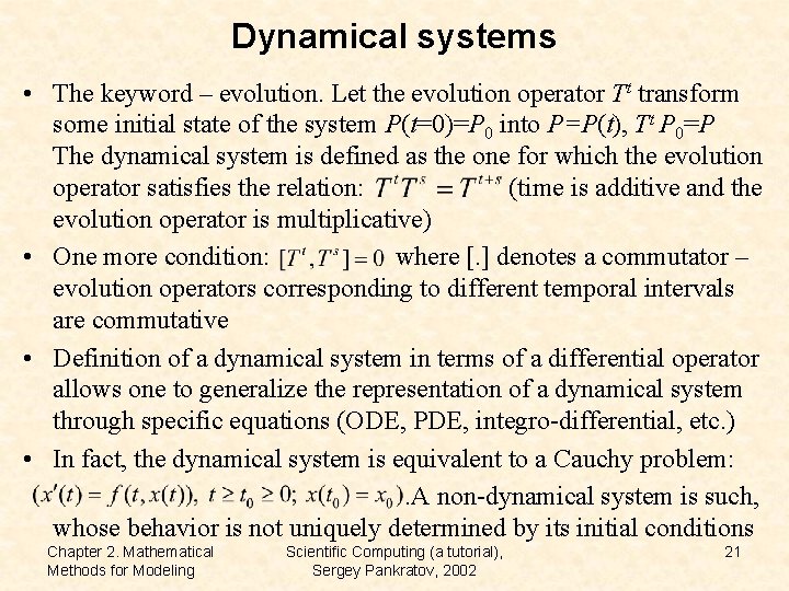
Dynamical systems • The keyword – evolution. Let the evolution operator Tt transform some initial state of the system P(t=0)=P 0 into P=P(t), Tt P 0=P The dynamical system is defined as the one for which the evolution operator satisfies the relation: (time is additive and the evolution operator is multiplicative) • One more condition: where [. ] denotes a commutator – evolution operators corresponding to different temporal intervals are commutative • Definition of a dynamical system in terms of a differential operator allows one to generalize the representation of a dynamical system through specific equations (ODE, PDE, integro-differential, etc. ) • In fact, the dynamical system is equivalent to a Cauchy problem: . A non-dynamical system is such, whose behavior is not uniquely determined by its initial conditions Chapter 2. Mathematical Methods for Modeling Scientific Computing (a tutorial), Sergey Pankratov, 2002 21

The motivation – why bother? • Dynamical systems contain geometric information in the form of a vector field. Interpretation of this geometrical information is the primary means of grasping evolutionary equations. Dynamics is the geometry of behavior • Qualitative analysis of solutions of dynamical systems may provide better understanding than numerical and even analytical calculations • Quantitative investigation of dynamical systems can be readily accompanied by visualization • Asymptotic analysis and long-term numerical exploration: to find the maximal time step still ensuring the closure of the approximate solutions to the exact solution • The exact solution exists (Cauchy-Peano theorem), is unique and continuous on rhs and initial conditions under general assumptions Chapter 2. Mathematical Methods for Modeling Scientific Computing (a tutorial), Sergey Pankratov, 2002 22

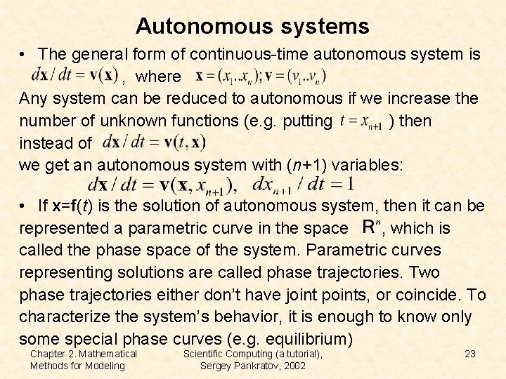
Autonomous systems • The general form of continuous-time autonomous system is , where Any system can be reduced to autonomous if we increase the number of unknown functions (e. g. putting ) then instead of we get an autonomous system with (n+1) variables: • If x=f(t) is the solution of autonomous system, then it can be represented a parametric curve in the space , which is called the phase space of the system. Parametric curves representing solutions are called phase trajectories. Two phase trajectories either don’t have joint points, or coincide. To characterize the system’s behavior, it is enough to know only some special phase curves (e. g. equilibrium) Chapter 2. Mathematical Methods for Modeling Scientific Computing (a tutorial), Sergey Pankratov, 2002 23

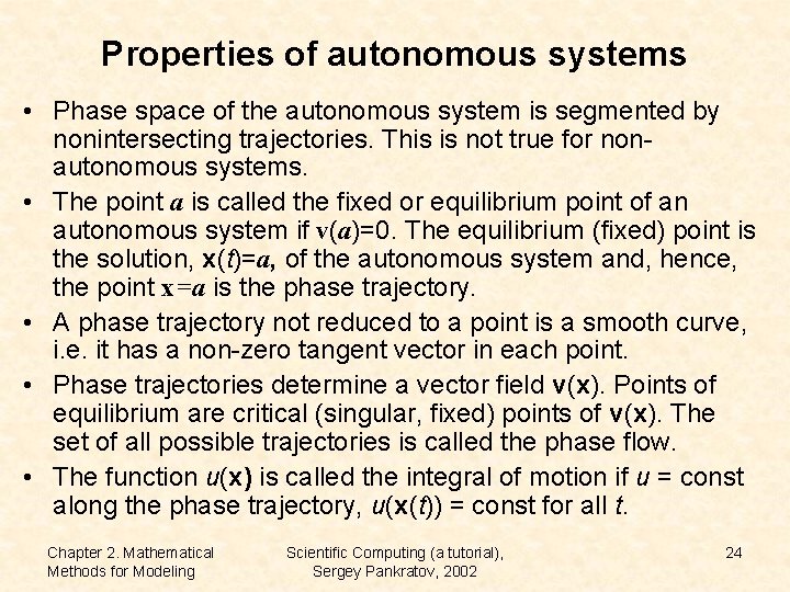
Properties of autonomous systems • Phase space of the autonomous system is segmented by nonintersecting trajectories. This is not true for nonautonomous systems. • The point a is called the fixed or equilibrium point of an autonomous system if v(a)=0. The equilibrium (fixed) point is the solution, x(t)=a, of the autonomous system and, hence, the point x=a is the phase trajectory. • A phase trajectory not reduced to a point is a smooth curve, i. e. it has a non-zero tangent vector in each point. • Phase trajectories determine a vector field v(x). Points of equilibrium are critical (singular, fixed) points of v(x). The set of all possible trajectories is called the phase flow. • The function u(x) is called the integral of motion if u = const along the phase trajectory, u(x(t)) = const for all t. Chapter 2. Mathematical Methods for Modeling Scientific Computing (a tutorial), Sergey Pankratov, 2002 24

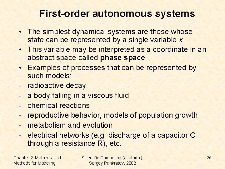
First-order autonomous systems • The simplest dynamical systems are those whose state can be represented by a single variable x • This variable may be interpreted as a coordinate in an abstract space called phase space • Examples of processes that can be represented by such models: - radioactive decay - a body falling in a viscous fluid - chemical reactions - reproductive behavior, models of population growth - metabolism and evolution - electrical networks (e. g. discharge of a capacitor C through a resistance R), etc. Chapter 2. Mathematical Methods for Modeling Scientific Computing (a tutorial), Sergey Pankratov, 2002 25

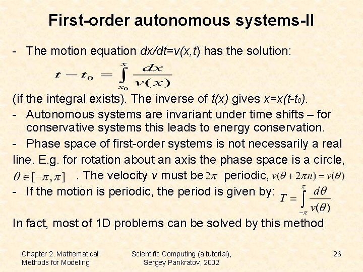
First-order autonomous systems-II - The motion equation dx/dt=v(x, t) has the solution: (if the integral exists). The inverse of t(x) gives x=x(t-t 0). - Autonomous systems are invariant under time shifts – for conservative systems this leads to energy conservation. - Phase space of first-order systems is not necessarily a real line. E. g. for rotation about an axis the phase space is a circle, . The velocity v must be periodic, - If the motion is periodic, the period is given by: In fact, most of 1 D problems can be solved by this method Chapter 2. Mathematical Methods for Modeling Scientific Computing (a tutorial), Sergey Pankratov, 2002 26

How to evaluate the behavior of first-order dynamical system without solving ODE? • The behavior of x(t) (in autonomous case x(t-t 0)) is controlled by zeroes of the velocity function v(x)=0, x=xm (equilibrium or fixed points). If the system is initially at xm, it remains there all the time. In all other initial points the state of the system must change. • Open intervals between two equilibrium (fixed) points, together with intervals that go from fixed points to infinity, are invariant sets, since a system whose evolution started between two fixed points cannot pass either of them. • There are two types of equilibrium points: stable and unstable. The equilibrium position a is stable when one can find the system near the equilibrium during the whole its evolution, provided it was sufficiently close to equilibrium at the initial moment (this is called Lyapunov stability) Chapter 2. Mathematical Methods for Modeling Scientific Computing (a tutorial), Sergey Pankratov, 2002 27

Rough classification of equilibrium points • There are only three basic types of equilibrium points of autonomous dynamical systems: sinks – nearby solutions converge to the equilibrium point sources – nearby solutions diverge nodes – any other behavior Let a be an equilibrium point for , then If , then a is a sink If , then a is a source If , then the equilibrium is indeterminate (node) Example: the logistic population model has a source at x=0 and a sink at x=1, which means that any nonzero initial population eventually comes to the normalized value x=1 Chapter 2. Mathematical Methods for Modeling Scientific Computing (a tutorial), Sergey Pankratov, 2002 28

Stability of first-order dynamical systems • A simpler stability test is as follows: a fixed point is stable if the velocity is decreasing when i. e. • One can approximate velocity near a stable equilibrium point with linear function so that the evolution here is described by where This solution shows explicitly that the trajectory does not reach the fixed point in finite time. Structurally unstable points: If x>0, then the system moves away from the equilibrium point and if x<0 then x(t) is moving towards it. The equilibrium (fixed) point is neither stable nor unstable. Small perturbation may radically change evolution of the system. Chapter 2. Mathematical Methods for Modeling Scientific Computing (a tutorial), Sergey Pankratov, 2002 29

The bugs are coming: population models - Imagine a bunch of insects reproducing generation after generation. Initially there were x 0 bugs, after i generations there will be xi of them (to bug us) - When a population in a given region is sufficiently large, it may be represented by a real continuous variable, x(t)>0. - If we assume that there is a maximum sustainable population, x=X, (an equilibrium state), and that the population dynamics can be described by a single equation dx/dt=v(x), then we can have a simple model v(x)=ax(X-x), a>0 and dx/dt=ax(X-x) – this is called the logistic model. The discrete alternative is the logistic map: xi+1=axi(1 -xi), 0<xi<1, a>0, i=0, 1, 2, . . The family of maps on the interval xi+1 = f(xi, a), of which the logistic map is the prime example, can be most effectively studied by using computer methods Chapter 2. Mathematical Methods for Modeling Scientific Computing (a tutorial), Sergey Pankratov, 2002 30

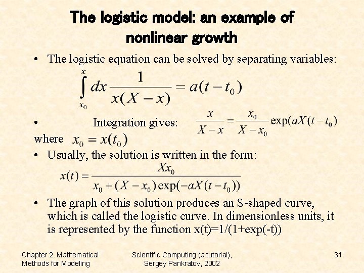
The logistic model: an example of nonlinear growth • The logistic equation can be solved by separating variables: • Integration gives: where • Usually, the solution is written in the form: • The graph of this solution produces an S-shaped curve, which is called the logistic curve. In dimensionless units, it is represented by the function x(t)=1/(1+exp(-t)) Chapter 2. Mathematical Methods for Modeling Scientific Computing (a tutorial), Sergey Pankratov, 2002 31

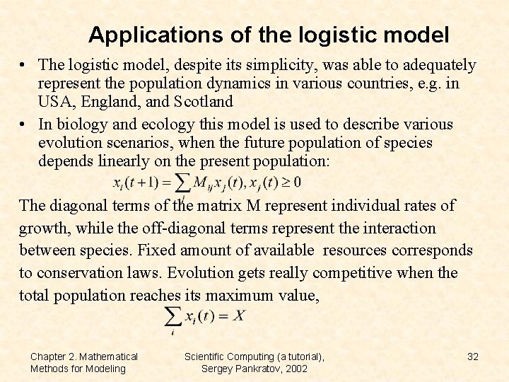
Applications of the logistic model • The logistic model, despite its simplicity, was able to adequately represent the population dynamics in various countries, e. g. in USA, England, and Scotland • In biology and ecology this model is used to describe various evolution scenarios, when the future population of species depends linearly on the present population: The diagonal terms of the matrix M represent individual rates of growth, while the off-diagonal terms represent the interaction between species. Fixed amount of available resources corresponds to conservation laws. Evolution gets really competitive when the total population reaches its maximum value, Chapter 2. Mathematical Methods for Modeling Scientific Computing (a tutorial), Sergey Pankratov, 2002 32

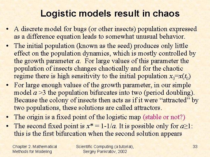
Logistic models result in chaos • A discrete model for bugs (or other insects) population expressed as a difference equation leads to somewhat unusual behavior. • The initial population (known as the seed) produces only little effect on the population dynamics, which is mostly controlled by the growth parameter a. For large values of this parameter the population of insects changes chaotically and for the chaotic regime there is high sensitivity to the initial population x 0=x(t 0) • For large enough values of the growth parameter, in our simple model a >3 the population bifurcates into two (period doubling). Because the colony of insects then acts as if it were “attracted” by two populations, these solutions are called attractors. • The origin is a fixed point of the logistic map (stable or not? ) • The second fixed point is x* = 1 -1/a. It is possible only for a≥ 1: this is the first bifurcation when the second solution appears Chapter 2. Mathematical Methods for Modeling Scientific Computing (a tutorial), Sergey Pankratov, 2002 33

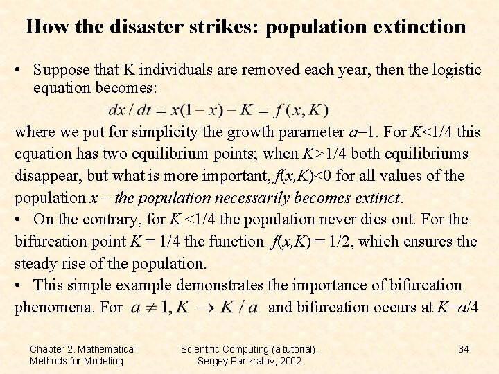
How the disaster strikes: population extinction • Suppose that K individuals are removed each year, then the logistic equation becomes: where we put for simplicity the growth parameter a=1. For K<1/4 this equation has two equilibrium points; when K>1/4 both equilibriums disappear, but what is more important, f(x, K)<0 for all values of the population x – the population necessarily becomes extinct. • On the contrary, for K <1/4 the population never dies out. For the bifurcation point K = 1/4 the function f(x, K) = 1/2, which ensures the steady rise of the population. • This simple example demonstrates the importance of bifurcation phenomena. For and bifurcation occurs at K=a/4 Chapter 2. Mathematical Methods for Modeling Scientific Computing (a tutorial), Sergey Pankratov, 2002 34

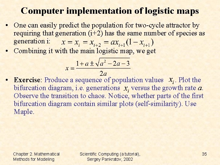
Computer implementation of logistic maps • One can easily predict the population for two-cycle attractor by requiring that generation (i+2) has the same number of species as generation i: • Combining it with the main logistic map, we get • Exercise: Produce a sequence of population values. Plot the bifurcation diagram, i. e. generations versus the growth rate a. Observe the transition to chaos. Notice, whether parts of the first bifurcation diagram contain similar plots (self-similarity). Use Maple. Chapter 2. Mathematical Methods for Modeling Scientific Computing (a tutorial), Sergey Pankratov, 2002 35

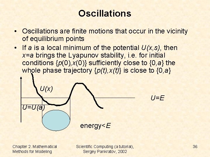
Oscillations • Oscillations are finite motions that occur in the vicinity of equilibrium points • If a is a local minimum of the potential U(x, s), then x=a brings the Lyapunov stability, i. e. for initial conditions {p(0), x(0)} sufficiently close to {0, a} the whole phase trajectory {p(t), x(t)} is close to {0, a} U(x) U=E U=U(a) energy<E Chapter 2. Mathematical Methods for Modeling Scientific Computing (a tutorial), Sergey Pankratov, 2002 36

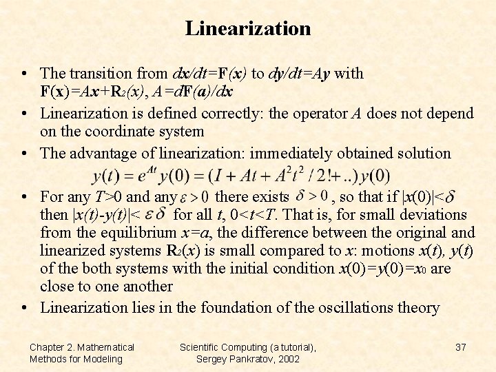
Linearization • The transition from dx/dt=F(x) to dy/dt=Ay with F(x)=Ax+R 2(x), A=d. F(a)/dx • Linearization is defined correctly: the operator A does not depend on the coordinate system • The advantage of linearization: immediately obtained solution • For any T>0 and any there exists , so that if |x(0)|< then |x(t)-y(t)|< for all t, 0<t<T. That is, for small deviations from the equilibrium x=a, the difference between the original and linearized systems R 2(x) is small compared to x: motions x(t), y(t) of the both systems with the initial condition x(0)=y(0)=x 0 are close to one another • Linearization lies in the foundation of the oscillations theory Chapter 2. Mathematical Methods for Modeling Scientific Computing (a tutorial), Sergey Pankratov, 2002 37

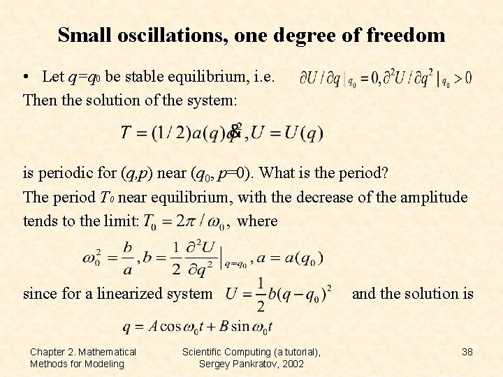
Small oscillations, one degree of freedom • Let q=q 0 be stable equilibrium, i. e. Then the solution of the system: is periodic for (q, p) near (q 0, p=0). What is the period? The period T 0 near equilibrium, with the decrease of the amplitude tends to the limit: where since for a linearized system Chapter 2. Mathematical Methods for Modeling Scientific Computing (a tutorial), Sergey Pankratov, 2002 and the solution is 38

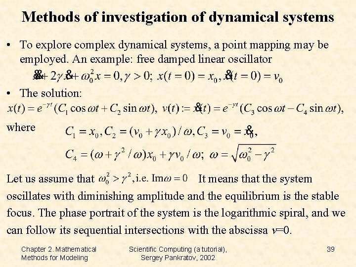
Methods of investigation of dynamical systems • To explore complex dynamical systems, a point mapping may be employed. An example: free damped linear oscillator • The solution: where Let us assume that It means that the system oscillates with diminishing amplitude and the equilibrium is the stable focus. The phase portrait of the system is the logarithmic spiral, and we can follow its sequential intersections with the abscissa v=0. Chapter 2. Mathematical Methods for Modeling Scientific Computing (a tutorial), Sergey Pankratov, 2002 39

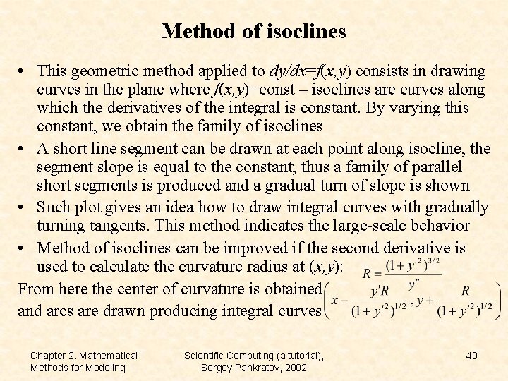
Method of isoclines • This geometric method applied to dy/dx=f(x, y) consists in drawing curves in the plane where f(x, y)=const – isoclines are curves along which the derivatives of the integral is constant. By varying this constant, we obtain the family of isoclines • A short line segment can be drawn at each point along isocline, the segment slope is equal to the constant; thus a family of parallel short segments is produced and a gradual turn of slope is shown • Such plot gives an idea how to draw integral curves with gradually turning tangents. This method indicates the large-scale behavior • Method of isoclines can be improved if the second derivative is used to calculate the curvature radius at (x, y): From here the center of curvature is obtained and arcs are drawn producing integral curves Chapter 2. Mathematical Methods for Modeling Scientific Computing (a tutorial), Sergey Pankratov, 2002 40

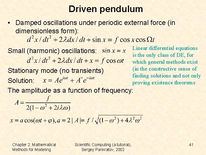
Driven pendulum • Damped oscillations under periodic external force (in dimensionless form): Small (harmonic) oscillations: Linear differential equations is the only class of DE, for which general methods exist (in the constructive sense of finding solutions and not only proving existence theorems Stationary mode (no transients) Solution: The amplitude as a function of frequency: Chapter 2. Mathematical Methods for Modeling Scientific Computing (a tutorial), Sergey Pankratov, 2002 41

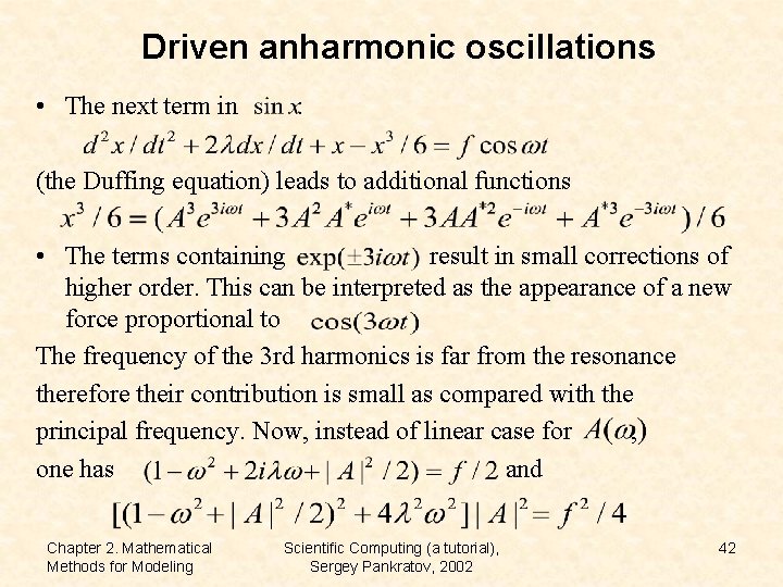
Driven anharmonic oscillations • The next term in : (the Duffing equation) leads to additional functions • The terms containing result in small corrections of higher order. This can be interpreted as the appearance of a new force proportional to The frequency of the 3 rd harmonics is far from the resonance therefore their contribution is small as compared with the principal frequency. Now, instead of linear case for , one has and Chapter 2. Mathematical Methods for Modeling Scientific Computing (a tutorial), Sergey Pankratov, 2002 42

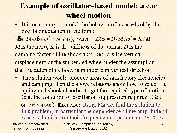
Example of oscillator-based model: a car wheel motion • It is customary to model the behavior of a car wheel by the oscillator equation in the form: where M is the mass, K is the stiffness of the spring, D is the damping factor of the shock absorber, x is the vertical displacement of the suspended wheel under the assumption that the automobile body is immobile in vertical direction • The solution would produce areas of satisfactory frequencies and damping, then the above relations show to select the spring and shock absorber to get the required type of motion (e. g. the condition of oscillation suppression requires or ). Exercise: Using Maple, find the solution to this problem, in particular the dependence of the amplitude of wheel vibrations on their frequency and parameters M, K, D Chapter 2. Mathematical Methods for Modeling Scientific Computing (a tutorial), Sergey Pankratov, 2002 43

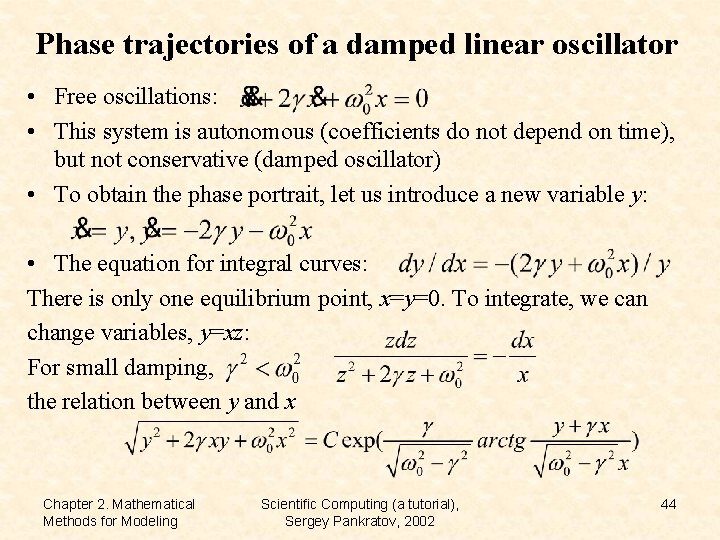
Phase trajectories of a damped linear oscillator • Free oscillations: • This system is autonomous (coefficients do not depend on time), but not conservative (damped oscillator) • To obtain the phase portrait, let us introduce a new variable y: • The equation for integral curves: There is only one equilibrium point, x=y=0. To integrate, we can change variables, y=xz: For small damping, the relation between y and x Chapter 2. Mathematical Methods for Modeling Scientific Computing (a tutorial), Sergey Pankratov, 2002 44

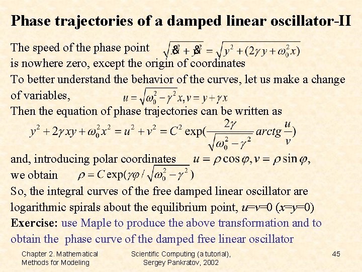
Phase trajectories of a damped linear oscillator-II The speed of the phase point is nowhere zero, except the origin of coordinates To better understand the behavior of the curves, let us make a change of variables, Then the equation of phase trajectories can be written as and, introducing polar coordinates we obtain So, the integral curves of the free damped linear oscillator are logarithmic spirals about the equilibrium point, u=v=0 (x=y=0) Exercise: use Maple to produce the above transformation and to obtain the phase curve of the damped free linear oscillator Chapter 2. Mathematical Methods for Modeling Scientific Computing (a tutorial), Sergey Pankratov, 2002 45

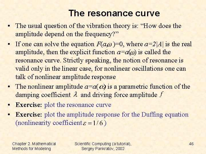
The resonance curve • The usual question of the vibration theory is: “How does the amplitude depend on the frequency? ” • If one can solve the equation F(a, )=0, where a=2|A| is the real amplitude, then the explicit function a=a( ) is called the resonance curve. Strictly speaking, the notion of resonance is valid only in the linear case, for nonlinear oscillations one can talk of nonlinear amplitude response • The nonlinear amplitude a=a( ) is a parametric function of the damping coefficient and driving force amplitude • Exercise: plot the resonance curve • Exercise: plot the amplitude response for the Duffing equation (nonlinearity coefficient ) Chapter 2. Mathematical Methods for Modeling Scientific Computing (a tutorial), Sergey Pankratov, 2002 46

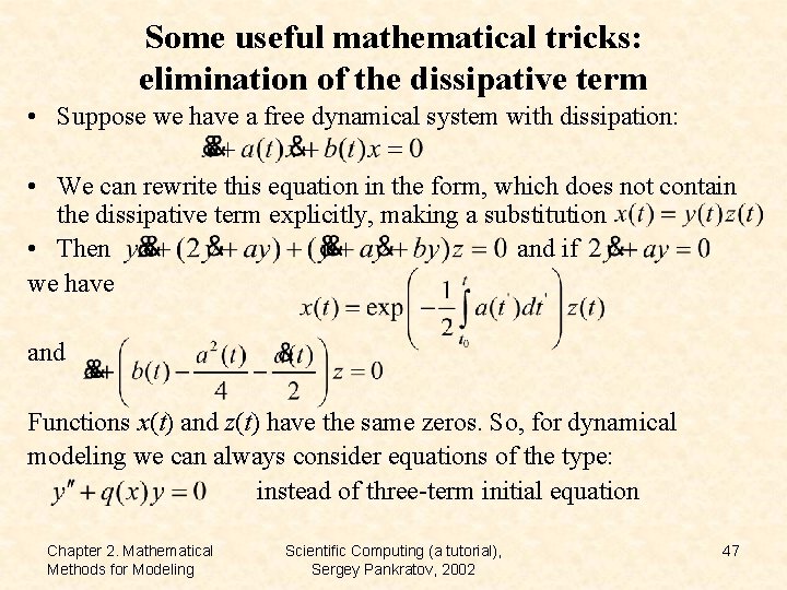
Some useful mathematical tricks: elimination of the dissipative term • Suppose we have a free dynamical system with dissipation: • We can rewrite this equation in the form, which does not contain the dissipative term explicitly, making a substitution • Then and if we have and Functions x(t) and z(t) have the same zeros. So, for dynamical modeling we can always consider equations of the type: instead of three-term initial equation Chapter 2. Mathematical Methods for Modeling Scientific Computing (a tutorial), Sergey Pankratov, 2002 47

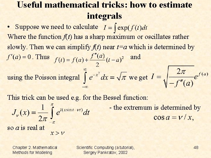
Useful mathematical tricks: how to estimate integrals • Suppose we need to calculate Where the function f(t) has a sharp maximum or oscillates rather slowly. Then we can simplify f(t) near t=a which is determined by. Thus and using the Poisson integral we get This trick can be used e. g. for the Bessel function: - the extremum is determined by so a is real at Chapter 2. Mathematical Methods for Modeling Scientific Computing (a tutorial), Sergey Pankratov, 2002 48

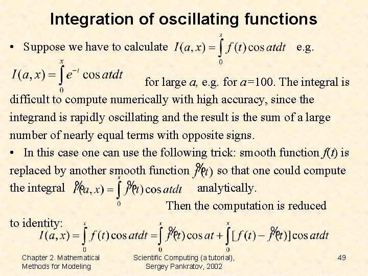
Integration of oscillating functions • Suppose we have to calculate e. g. for large a, e. g. for a=100. The integral is difficult to compute numerically with high accuracy, since the integrand is rapidly oscillating and the result is the sum of a large number of nearly equal terms with opposite signs. • In this case one can use the following trick: smooth function f(t) is replaced by another smooth function so that one could compute the integral analytically. Then the computation is reduced to identity: Chapter 2. Mathematical Methods for Modeling Scientific Computing (a tutorial), Sergey Pankratov, 2002 49

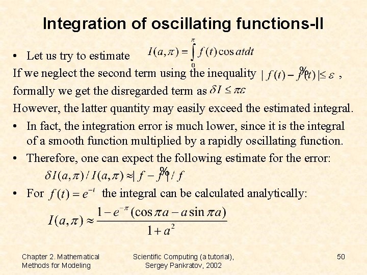
Integration of oscillating functions-II • Let us try to estimate If we neglect the second term using the inequality , formally we get the disregarded term as However, the latter quantity may easily exceed the estimated integral. • In fact, the integration error is much lower, since it is the integral of a smooth function multiplied by a rapidly oscillating function. • Therefore, one can expect the following estimate for the error: • For Chapter 2. Mathematical Methods for Modeling the integral can be calculated analytically: Scientific Computing (a tutorial), Sergey Pankratov, 2002 50

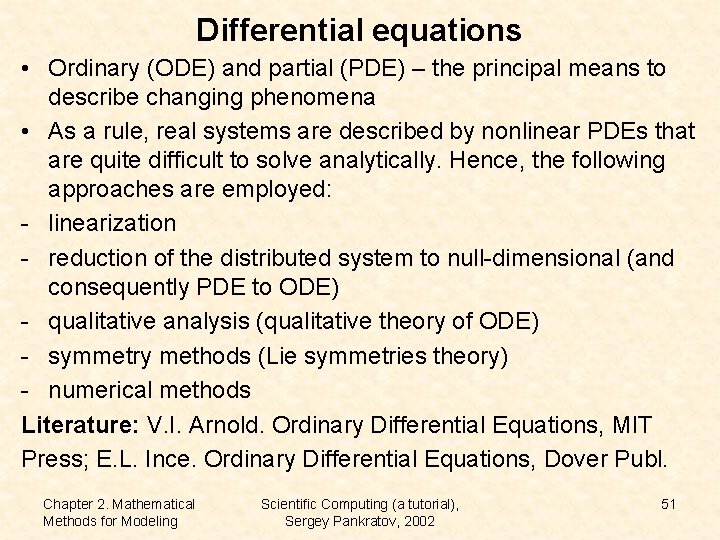
Differential equations • Ordinary (ODE) and partial (PDE) – the principal means to describe changing phenomena • As a rule, real systems are described by nonlinear PDEs that are quite difficult to solve analytically. Hence, the following approaches are employed: - linearization - reduction of the distributed system to null-dimensional (and consequently PDE to ODE) - qualitative analysis (qualitative theory of ODE) - symmetry methods (Lie symmetries theory) - numerical methods Literature: V. I. Arnold. Ordinary Differential Equations, MIT Press; E. L. Ince. Ordinary Differential Equations, Dover Publ. Chapter 2. Mathematical Methods for Modeling Scientific Computing (a tutorial), Sergey Pankratov, 2002 51

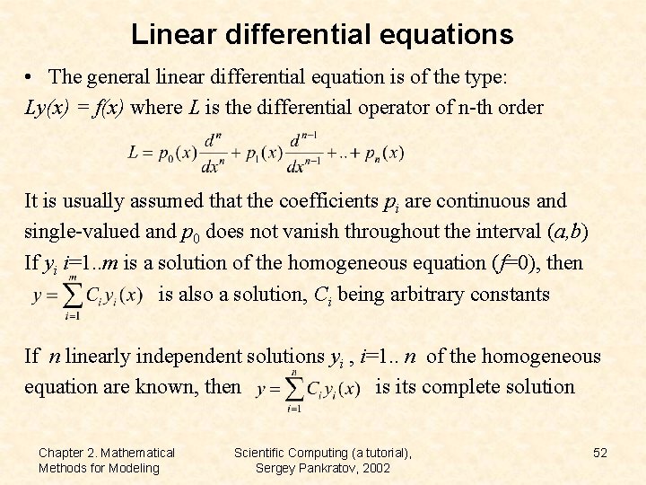
Linear differential equations • The general linear differential equation is of the type: Ly(x) = f(x) where L is the differential operator of n-th order It is usually assumed that the coefficients pi are continuous and single-valued and p 0 does not vanish throughout the interval (a, b) If yi i=1. . m is a solution of the homogeneous equation (f=0), then is also a solution, Ci being arbitrary constants If n linearly independent solutions yi , i=1. . n of the homogeneous equation are known, then is its complete solution Chapter 2. Mathematical Methods for Modeling Scientific Computing (a tutorial), Sergey Pankratov, 2002 52

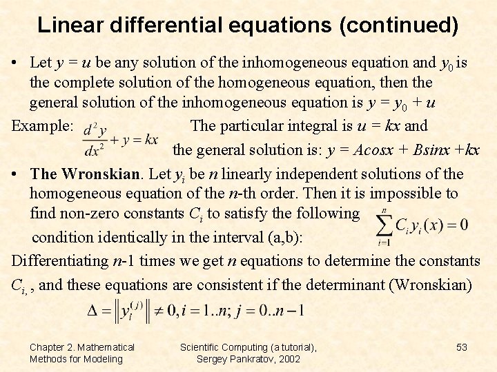
Linear differential equations (continued) • Let y = u be any solution of the inhomogeneous equation and y 0 is the complete solution of the homogeneous equation, then the general solution of the inhomogeneous equation is y = y 0 + u Example: The particular integral is u = kx and the general solution is: y = Acosx + Bsinx +kx • The Wronskian. Let yi be n linearly independent solutions of the homogeneous equation of the n-th order. Then it is impossible to find non-zero constants Ci to satisfy the following condition identically in the interval (a, b): Differentiating n-1 times we get n equations to determine the constants Ci, , and these equations are consistent if the determinant (Wronskian) Chapter 2. Mathematical Methods for Modeling Scientific Computing (a tutorial), Sergey Pankratov, 2002 53

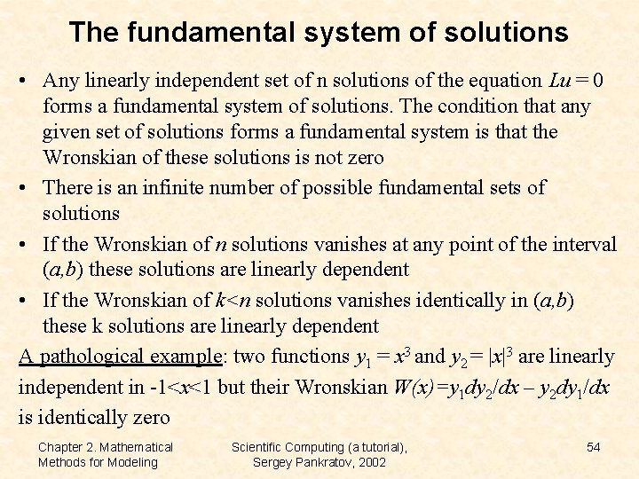
The fundamental system of solutions • Any linearly independent set of n solutions of the equation Lu = 0 forms a fundamental system of solutions. The condition that any given set of solutions forms a fundamental system is that the Wronskian of these solutions is not zero • There is an infinite number of possible fundamental sets of solutions • If the Wronskian of n solutions vanishes at any point of the interval (a, b) these solutions are linearly dependent • If the Wronskian of k<n solutions vanishes identically in (a, b) these k solutions are linearly dependent A pathological example: two functions y 1 = x 3 and y 2 = |x|3 are linearly independent in -1<x<1 but their Wronskian W(x)=y 1 dy 2/dx – y 2 dy 1/dx is identically zero Chapter 2. Mathematical Methods for Modeling Scientific Computing (a tutorial), Sergey Pankratov, 2002 54

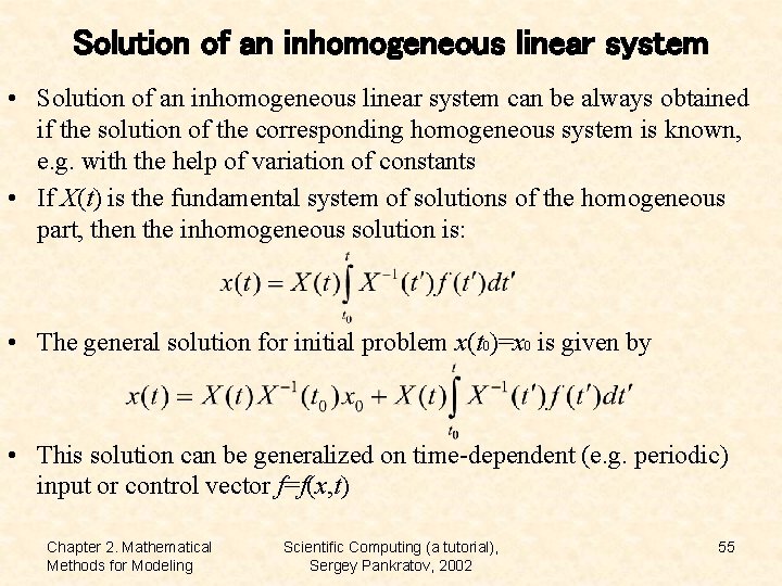
Solution of an inhomogeneous linear system • Solution of an inhomogeneous linear system can be always obtained if the solution of the corresponding homogeneous system is known, e. g. with the help of variation of constants • If X(t) is the fundamental system of solutions of the homogeneous part, then the inhomogeneous solution is: • The general solution for initial problem x(t 0)=x 0 is given by • This solution can be generalized on time-dependent (e. g. periodic) input or control vector f=f(x, t) Chapter 2. Mathematical Methods for Modeling Scientific Computing (a tutorial), Sergey Pankratov, 2002 55

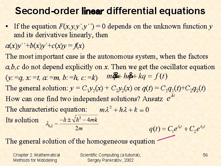
Second-order linear differential equations • If the equation F(x, y, y´´) = 0 depends on the unknown function y and its derivatives linearly, then a(x)y´´+b(x)y´+c(x)y = f(x) The most important case is the autonomous system, when the factors a, b, c do not depend explicitly on x. Then we get the oscillator equation (y: =q, x: =t, a: =m, b: =h, c: =k) The general solution: y = C 1 y 1(x) + C 2 y 2(x) or q(t) = C 1 q 1(t)+C 2 q 2(t) How can one find two independent solutions? Ansatz The characteristic equation: Its solution The general solution of the homogeneous equation Chapter 2. Mathematical Methods for Mdodeling Scientific Computing (a tutorial), Sergey Pankratov, 2002 56

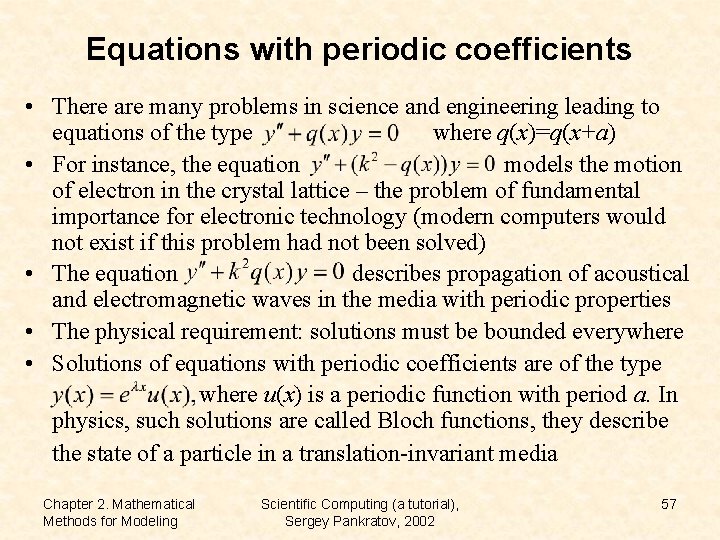
Equations with periodic coefficients • There are many problems in science and engineering leading to equations of the type where q(x)=q(x+a) • For instance, the equation models the motion of electron in the crystal lattice – the problem of fundamental importance for electronic technology (modern computers would not exist if this problem had not been solved) • The equation describes propagation of acoustical and electromagnetic waves in the media with periodic properties • The physical requirement: solutions must be bounded everywhere • Solutions of equations with periodic coefficients are of the type where u(x) is a periodic function with period a. In physics, such solutions are called Bloch functions, they describe the state of a particle in a translation-invariant media Chapter 2. Mathematical Methods for Modeling Scientific Computing (a tutorial), Sergey Pankratov, 2002 57

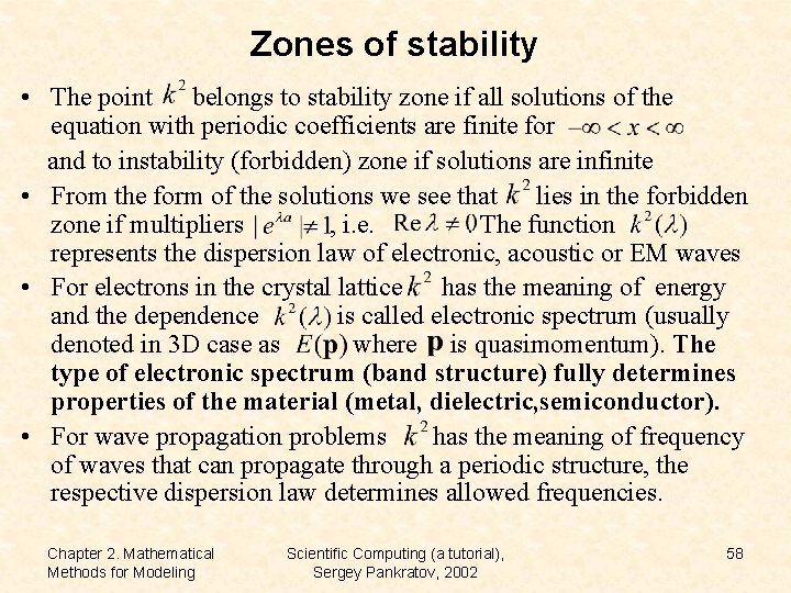
Zones of stability • The point belongs to stability zone if all solutions of the equation with periodic coefficients are finite for and to instability (forbidden) zone if solutions are infinite • From the form of the solutions we see that lies in the forbidden zone if multipliers , i. e. . The function represents the dispersion law of electronic, acoustic or EM waves • For electrons in the crystal lattice has the meaning of energy and the dependence is called electronic spectrum (usually denoted in 3 D case as where is quasimomentum). The type of electronic spectrum (band structure) fully determines properties of the material (metal, dielectric, semiconductor). • For wave propagation problems has the meaning of frequency of waves that can propagate through a periodic structure, the respective dispersion law determines allowed frequencies. Chapter 2. Mathematical Methods for Modeling Scientific Computing (a tutorial), Sergey Pankratov, 2002 58

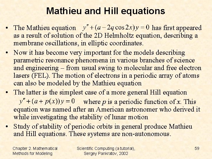
Mathieu and Hill equations • The Mathieu equation has first appeared as a result of solution of the 2 D Helmholtz equation, describing a membrane oscillations, in elliptic coordinates. • Now it has become very important for the models describing parametric resonance phenomena in various branches of science and engineering – from usual swing to molecular and free electron lasers (FEL). The motion of electrons in a periodic array of atoms can also be modeled by the Mathieu equation • The latter is the simplest case of a more general Hill equation where p is a periodic function of x. This equation was named after an American astronomer who derived it while investigating the stability of lunar motion • Study of stability of periodic orbits in general produce Mathieu and Hill equations. These systems are non-autonomous. Chapter 2. Mathematical Methods for Modeling Scientific Computing (a tutorial), Sergey Pankratov, 2002 59

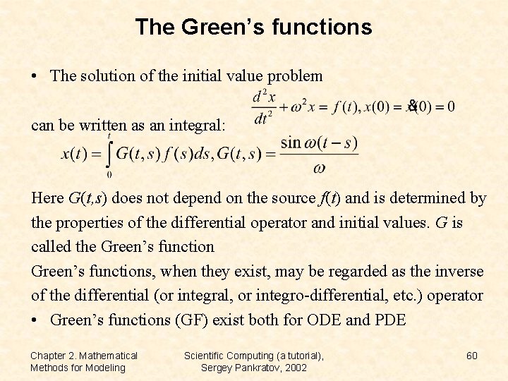
The Green’s functions • The solution of the initial value problem can be written as an integral: Here G(t, s) does not depend on the source f(t) and is determined by the properties of the differential operator and initial values. G is called the Green’s functions, when they exist, may be regarded as the inverse of the differential (or integral, or integro-differential, etc. ) operator • Green’s functions (GF) exist both for ODE and PDE Chapter 2. Mathematical Methods for Modeling Scientific Computing (a tutorial), Sergey Pankratov, 2002 60

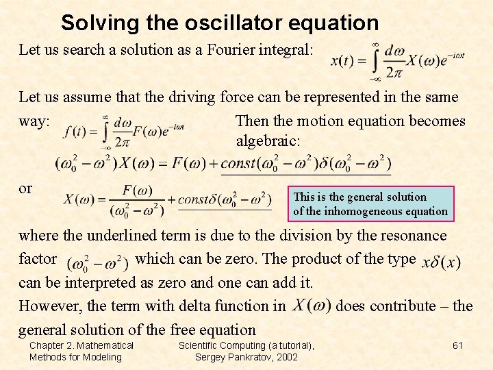
Solving the oscillator equation Let us search a solution as a Fourier integral: Let us assume that the driving force can be represented in the same way: Then the motion equation becomes algebraic: or This is the general solution of the inhomogeneous equation where the underlined term is due to the division by the resonance factor which can be zero. The product of the type can be interpreted as zero and one can add it. However, the term with delta function in does contribute – the general solution of the free equation Chapter 2. Mathematical Methods for Modeling Scientific Computing (a tutorial), Sergey Pankratov, 2002 61

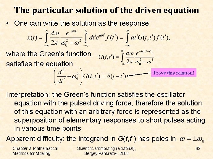
The particular solution of the driven equation • One can write the solution as the response where the Green’s function, satisfies the equation Prove this relation! Interpretation: the Green’s function satisfies the oscillator equation with the pulsed driving force, therefore the solution of this equation with an arbitrary force is represented as the superposition of elementary responses to short pulses acting in various time points Apparent difficulty: the integrand in G(t, t´) has poles in Chapter 2. Mathematical Methods for Mdeling Scientific Computing (a tutorial), Sergey Pankratov, 2002 62

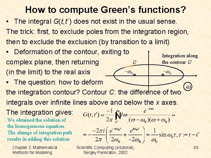
How to compute Green’s functions? • The integral G(t, t´) does not exist in the usual sense. The trick: first, to exclude poles from the integration region, then to exclude the exclusion (by transition to a limit) • Deformation of the contour, exiting to Integration along the contour C C complex plane, then returning (in the limit) to the real axis • The question: how to deform the integration contour? Contour C: the difference of two integrals over infinite lines above and below the x axes. The integration gives: We obtained the solution of the homogeneous equation. The change of integration path results in adding this solution Chapter 2. Mathematical Methods for Modeling Scientific Computing (a tutorial), Sergey Pankratov, 2002 63

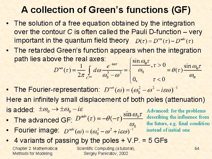
A collection of Green’s functions (GF) • The solution of a free equation obtained by the integration over the contour C is often called the Pauli D-function – very important in the quantum field theory • The retarded Green’s function appears when the integration path lies above the real axes: • The Fourier-representation: Here an infinitely small displacement of both poles (attenuation) is added: Advanced: for the problems describing the influence from • The advanced GF: the future, e. g. final condition instead of initial one • Fourier image: • 4 variants of passing by the poles + V. P. = 5 GFs Chapter 2. Mathematical Methods for Modeling Scientific Computing (a tutorial), Sergey Pankratov, 2002 64

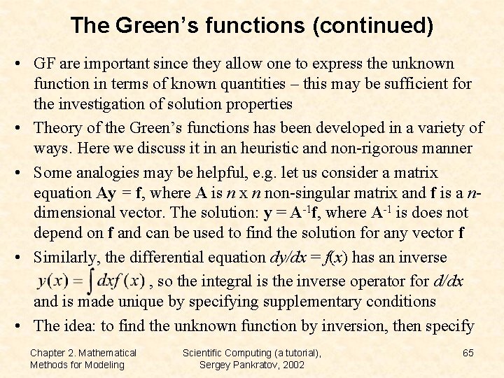
The Green’s functions (continued) • GF are important since they allow one to express the unknown function in terms of known quantities – this may be sufficient for the investigation of solution properties • Theory of the Green’s functions has been developed in a variety of ways. Here we discuss it in an heuristic and non-rigorous manner • Some analogies may be helpful, e. g. let us consider a matrix equation Ay = f, where A is n x n non-singular matrix and f is a ndimensional vector. The solution: y = A-1 f, where A-1 is does not depend on f and can be used to find the solution for any vector f • Similarly, the differential equation dy/dx = f(x) has an inverse , so the integral is the inverse operator for d/dx and is made unique by specifying supplementary conditions • The idea: to find the unknown function by inversion, then specify Chapter 2. Mathematical Methods for Modeling Scientific Computing (a tutorial), Sergey Pankratov, 2002 65

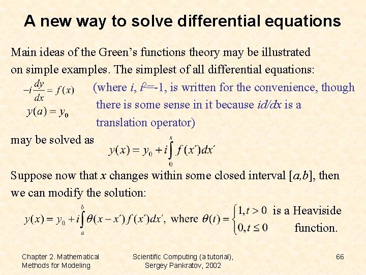
A new way to solve differential equations Main ideas of the Green’s functions theory may be illustrated on simple examples. The simplest of all differential equations: (where i, i 2=-1, is written for the convenience, though there is some sense in it because id/dx is a translation operator) may be solved as Suppose now that x changes within some closed interval [a, b], then we can modify the solution: is a Heaviside function. Chapter 2. Mathematical Methods for Modeling Scientific Computing (a tutorial), Sergey Pankratov, 2002 66

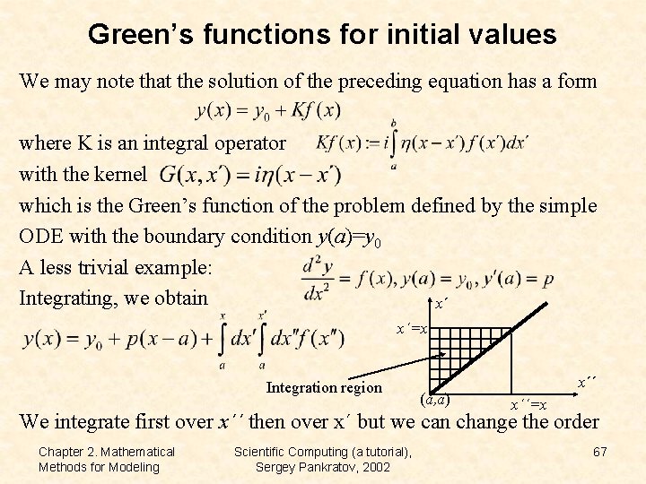
Green’s functions for initial values We may note that the solution of the preceding equation has a form where K is an integral operator with the kernel which is the Green’s function of the problem defined by the simple ODE with the boundary condition y(a)=y 0 A less trivial example: Integrating, we obtain x´ x´=x Integration region (a, a) x´´=x We integrate first over x´´ then over x´ but we can change the order Chapter 2. Mathematical Methods for Modeling Scientific Computing (a tutorial), Sergey Pankratov, 2002 67

Green’s functions for boundary values We get: Restricting x to the interval [a, b], we may write where is the Green’s function for the operator d 2/dx 2 with the above supplementary (initial) conditions. The general solution: where C 1, C 2 can be determined from boundary conditions Exercise: find the solution for boundary conditions y(0)=y 0, y(1)=y 1 Chapter 2. Mathematical Methods for Modeling Scientific Computing (a tutorial), Sergey Pankratov, 2002 68

Chapter 3. Numerical Methods for Modeling Some generalities: • There are tons of books on numerical methods Roughly, two groups of information sources and their recipients 1) numerical mathematics as a scientific subject 2) numerical mathematics as a working tool This chapter is oriented at 2): using general numerical methods to solve applied problems • Therefore – ultimate generality and rigour are unnecessary Functions are assumed smooth, meaning “finite together with all the derivatives of the order to be used in the specific case”, where needed From a physicist’s point of view, numerical techniques seem to be closer to experimental science than to idealized mathematical constructions: 1) it’s an art where the result justifies the means; 2) it’s a team game – interdisciplinary sport Chapter 3. Numerical Methods for Modeling Scientific Computing (a tutorial), Sergey Pankratov, 2002 69

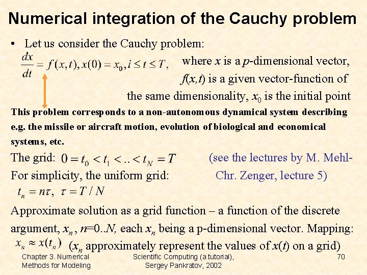
Numerical integration of the Cauchy problem • Let us consider the Cauchy problem: where x is a p-dimensional vector, f(x, t) is a given vector-function of the same dimensionality, x 0 is the initial point This problem corresponds to a non-autonomous dynamical system describing e. g. the missile or aircraft motion, evolution of biological and economical systems, etc. The grid: For simplicity, the uniform grid: (see the lectures by M. Mehl. Chr. Zenger, lecture 5) Approximate solution as a grid function – a function of the discrete argument, xn , n=0. . N, each xn being a p-dimensional vector. Mapping: (xn approximately represent the values of x(t) on a grid) Chapter 3. Numerical Methods for Modeling Scientific Computing (a tutorial), Sergey Pankratov, 2002 70

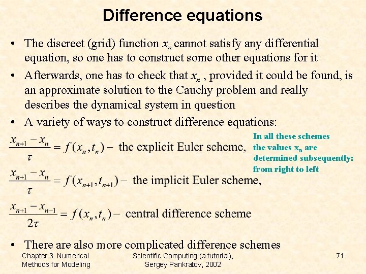
Difference equations • The discreet (grid) function xn cannot satisfy any differential equation, so one has to construct some other equations for it • Afterwards, one has to check that xn , provided it could be found, is an approximate solution to the Cauchy problem and really describes the dynamical system in question • A variety of ways to construct difference equations: In all these schemes the values xn are determined subsequently: from right to left • There also more complicated difference schemes Chapter 3. Numerical Methods for Modeling Scientific Computing (a tutorial), Sergey Pankratov, 2002 71

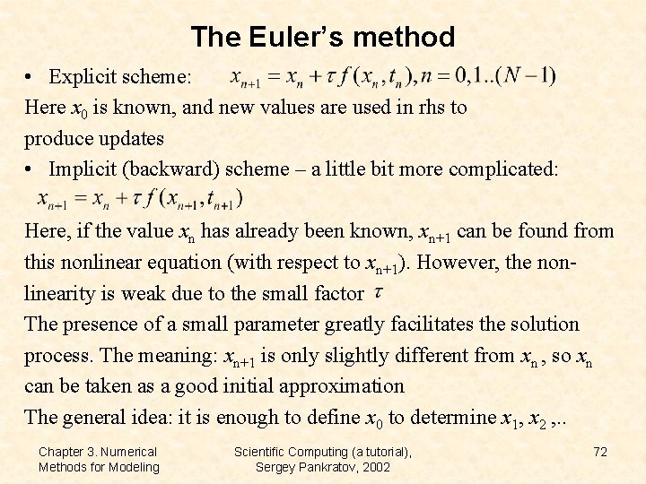
The Euler’s method • Explicit scheme: Here x 0 is known, and new values are used in rhs to produce updates • Implicit (backward) scheme – a little bit more complicated: Here, if the value xn has already been known, xn+1 can be found from this nonlinear equation (with respect to xn+1). However, the nonlinearity is weak due to the small factor The presence of a small parameter greatly facilitates the solution process. The meaning: xn+1 is only slightly different from xn , so xn can be taken as a good initial approximation The general idea: it is enough to define x 0 to determine x 1, x 2 , . . Chapter 3. Numerical Methods for Modeling Scientific Computing (a tutorial), Sergey Pankratov, 2002 72

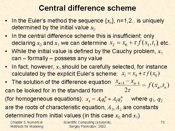
Central difference scheme • In the Euler’s method the sequence {xn}, n=1, 2. . is uniquely determined by the initial value x 0 • In the central difference scheme this is insufficient: only declaring x 0 and x 1 we can determine , etc. • While the initial value is defined by the Cauchy problem, x 1 can – formally – possess any value • In fact, however, x 1 should be carefully selected, for instance calculated by the explicit Euler’s scheme: • The solution of the difference equation can be looked for in the standard form (for homogeneous equations): where q 1, q 2 are the roots of characteristic equation, A 1, A 2 are constants determined from initial values (in this case x 0 and x 1) Chapter 3. Numerical Methods for Modeling Scientific Computing (a tutorial), Sergey Pankratov, 2002 73

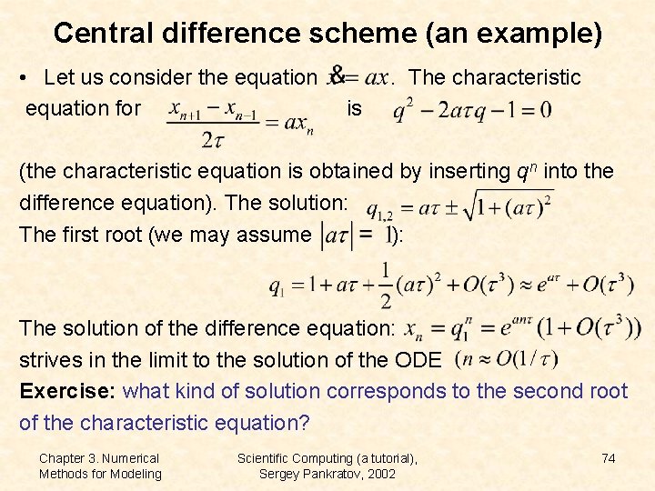
Central difference scheme (an example) • Let us consider the equation for . The characteristic is (the characteristic equation is obtained by inserting qn into the difference equation). The solution: The first root (we may assume ): The solution of the difference equation: strives in the limit to the solution of the ODE Exercise: what kind of solution corresponds to the second root of the characteristic equation? Chapter 3. Numerical Methods for Modeling Scientific Computing (a tutorial), Sergey Pankratov, 2002 74

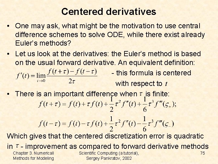
Centered derivatives • One may ask, what might be the motivation to use central difference schemes to solve ODE, while there exist already Euler’s methods? • Let us look at the derivatives: the Euler’s method is based on the usual forward derivative. An equivalent definition: - this formula is centered with respect to t • There is an important difference when is finite: Which gives that the centered discretization error is quadratic in - improvement as compared to forward derivative methods Chapter 3. Numericall Methods for Modeling Scientific Computing (a tutorial), Sergey Pankratov, 2002 75

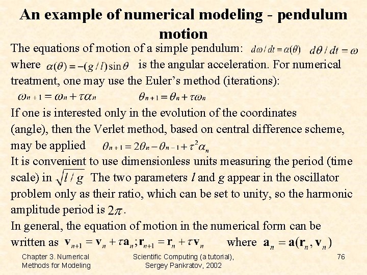
An example of numerical modeling - pendulum motion The equations of motion of a simple pendulum: where is the angular acceleration. For numerical treatment, one may use the Euler’s method (iterations): If one is interested only in the evolution of the coordinates (angle), then the Verlet method, based on central difference scheme, may be applied It is convenient to use dimensionless units measuring the period (time scale) in The two parameters l and g appear in the oscillator problem only as their ratio, which can be set to unity, so the harmonic amplitude period is. In general, the equation of motion in the numerical form can be written as where Chapter 3. Numerical Methods for Modeling Scientific Computing (a tutorial), Sergey Pankratov, 2002 76

Chapter 4. Examples of Mathematical Models • The chapter contains examples of mathematical methods, numerical techniques and computer algebra manipulations applied to mathematical models frequently encountered in various branches of science and engineering • Most of the models have been imported from physics and applied for scientific and engineering problems. • One may use the term “compumatical methods” stressing the merge of analytical and computer techniques. • A mathematical model is not uniquely determined by investigated object or situation. Selection of the model is dictated by accuracy requirements. Examples - a table: rectangular or not; ballistics: influence of the atmosphere; atom: finite dimensions of nucleus; motion of a satellite: nonspheroidal shape of the Earth Chapter 4. Examples of Mathematical Models Scientific Computing (a tutorial), Sergey Pankratov, 2002 77

The arms race • Let us imagine two hypothetical adversaries accumulating e. g. weapons of mass destruction, W 1 and W 2 being the total quantities of such weapons owned by each country. By W 1 and W 2 one can also imply the quantities of fission material (Plutonium), number of warheads, or deadly chemical/biological agents, • The simplest model is based on assumption that the temporal variation of W 1 and W 2 is proportional to the following factors: - intelligence data on the accumulated weapons by the adversary - ageing with speed bi , i=1, 2, of already produced and deployed weapons - the degree of mutual distrust and political tension, characterized by a two-component function ci(t), i=1, 2, can be obtained from another dynamical model (describing political interaction and competition) Chapter 4. Examples of Mathematical Models Scientific Computing (a tutorial), Sergey Pankratov, 2002 78

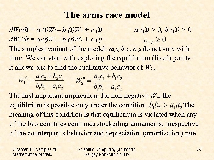
The arms race model d. W 1/dt = a 1(t)W 2 – b 1(t)W 1 + c 1(t) a 1, 2(t) > 0, b 1, 2(t) > 0 d. W 2/dt = a 2(t)W 1 – b 2(t)W 2 + c 2(t) The simplest variant of the model: a 1, 2, b 1, 2 , c 1, 2 do not vary with time. We can start with exploring the equilibrium (fixed) points: it allows one to find the qualitative behavior of W 1, 2 The first important implication: for non-negative W 1, 2 the equilibrium is possible only under the condition The meaning of this condition is that equilibrium is violated when any of the two countries continues stockpiling armaments, irrespective of the counterpart’s behavior and depreciation (amortization) rate Chapter 4. Examples of Mathematical Models Scientific Computing (a tutorial), Sergey Pankratov, 2002 79

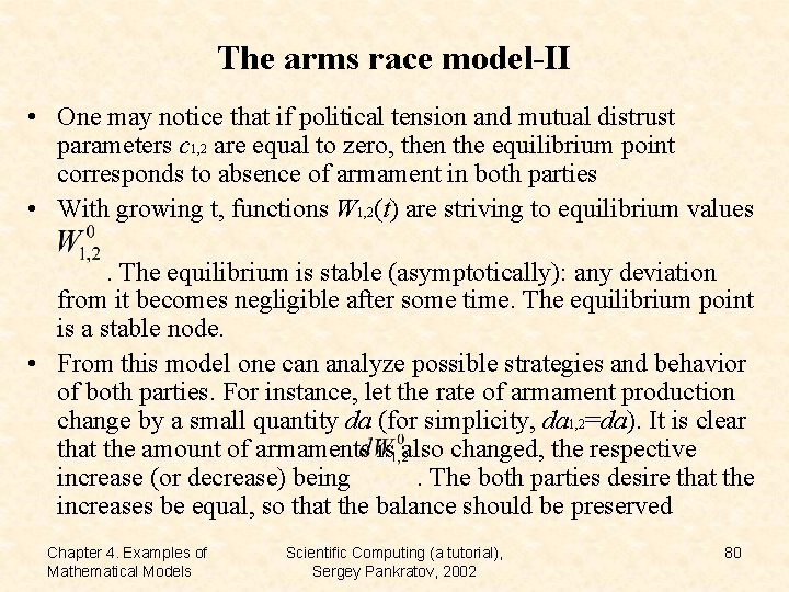
The arms race model-II • One may notice that if political tension and mutual distrust parameters c 1, 2 are equal to zero, then the equilibrium point corresponds to absence of armament in both parties • With growing t, functions W 1, 2(t) are striving to equilibrium values. The equilibrium is stable (asymptotically): any deviation from it becomes negligible after some time. The equilibrium point is a stable node. • From this model one can analyze possible strategies and behavior of both parties. For instance, let the rate of armament production change by a small quantity da (for simplicity, da 1, 2=da). It is clear that the amount of armaments is also changed, the respective increase (or decrease) being. The both parties desire that the increases be equal, so that the balance should be preserved Chapter 4. Examples of Mathematical Models Scientific Computing (a tutorial), Sergey Pankratov, 2002 80

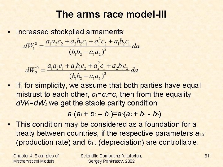
The arms race model-III • Increased stockpiled armaments: • If, for simplicity, we assume that both parties have equal mistrust to each other, c 1=c 2=c, then from the equality d. W 1=d. W 2 we get the stable parity condition: a 1(a 1 + b 2 – b 1)=a 2(a 2 + b 1 - b 2) • This condition may be considered as a foundation for a treaty between countries, if the respective parameters a 1, 2 (production rate) and b 1, 2 (depreciation) are controllable. Chapter 4. Examples of Mathematical Models Scientific Computing (a tutorial), Sergey Pankratov, 2002 81

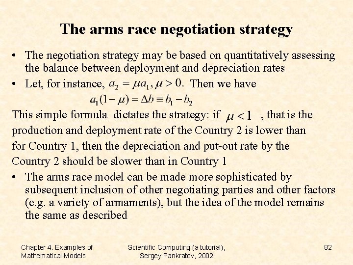
The arms race negotiation strategy • The negotiation strategy may be based on quantitatively assessing the balance between deployment and depreciation rates • Let, for instance, Then we have This simple formula dictates the strategy: if , that is the production and deployment rate of the Country 2 is lower than for Country 1, then the depreciation and put-out rate by the Country 2 should be slower than in Country 1 • The arms race model can be made more sophisticated by subsequent inclusion of other negotiating parties and other factors (e. g. a variety of armaments), but the idea of the model remains the same as described Chapter 4. Examples of Mathematical Models Scientific Computing (a tutorial), Sergey Pankratov, 2002 82

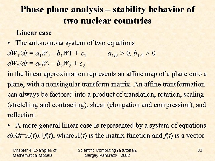
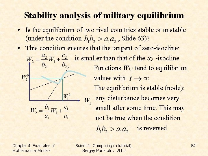
Phase plane analysis – stability behavior of two nuclear countries Linear case • The autonomous system of two equations d. W 1/dt = a 1 W 2 – b 1 W 1 + c 1 a 1, 2 > 0, b 1, 2 > 0 d. W 2/dt = a 2 W 1 – b 2 W 2 + c 2 in the linear approximation represents an affine map of a plane onto a plane, with a nonsingular transform matrix. An affine transformation can always be factored into a product of translation, rotation, scaling (stretching and contracting), shear (elongation and compression), and reflection. • A more general linear case is represented by a system of equations dx/dt=A(t)x+f(t), where A(t) is the matrix function and f(t) is a vector Chapter 4. Examples of Mathematical Models Scientific Computing (a tutorial), Sergey Pankratov, 2002 83

Stability analysis of military equilibrium • Is the equilibrium of two rival countries stable or unstable (under the condition , Slide 63)? • This condition ensures that the tangent of zero-isocline: is smaller than that of the -isocline Functions W 1, 2 tend to equilibrium values with The equilibrium is stable (node): any disturbance becomes very small after some time. This may not be true when the condition is reversed Chapter 4. Examples of Mathematical Models Scientific Computing (a tutorial), Sergey Pankratov, 2002 84

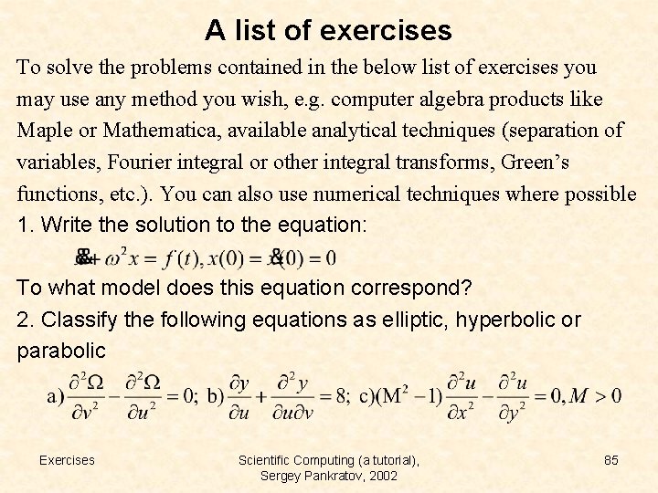
A list of exercises To solve the problems contained in the below list of exercises you may use any method you wish, e. g. computer algebra products like Maple or Mathematica, available analytical techniques (separation of variables, Fourier integral or other integral transforms, Green’s functions, etc. ). You can also use numerical techniques where possible 1. Write the solution to the equation: To what model does this equation correspond? 2. Classify the following equations as elliptic, hyperbolic or parabolic Exercises Scientific Computing (a tutorial), Sergey Pankratov, 2002 85

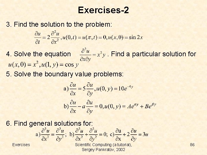
Exercises-2 3. Find the solution to the problem: 4. Solve the equation . Find a particular solution for 5. Solve the boundary value problems: 6. Find general solutions for: Exercises Scientific Computing (a tutorial), Sergey Pankratov, 2002 86

Exercises-3 7. Let A be an n x n matrix whose entries depend smoothly on a parameter t. Are the following relations correct? 8. Calculate eigenvalues and eigenvectors of the matrix A: a) Are the eigenvectors orthogonal? b) Can they form a basis in some space? c) Find a unitary matrix U diagonalizing A 9. Show that the 1 D wave equation is invariant under the transformation Chapter 1. Mathematical Methods with Maple Scientific Computing (a tutorial), Sergey Pankratov, 2002 87

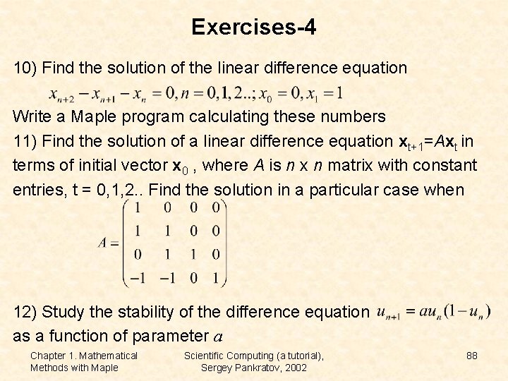
Exercises-4 10) Find the solution of the linear difference equation Write a Maple program calculating these numbers 11) Find the solution of a linear difference equation xt+1=Axt in terms of initial vector x 0 , where A is n x n matrix with constant entries, t = 0, 1, 2. . Find the solution in a particular case when 12) Study the stability of the difference equation as a function of parameter a Chapter 1. Mathematical Methods with Maple Scientific Computing (a tutorial), Sergey Pankratov, 2002 88

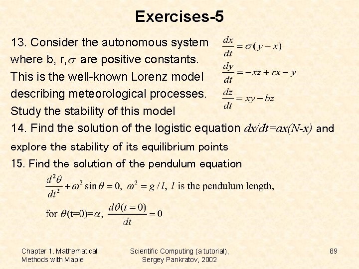
Exercises-5 13. Consider the autonomous system where b, r, are positive constants. This is the well-known Lorenz model describing meteorological processes. Study the stability of this model 14. Find the solution of the logistic equation dx/dt=ax(N-x) and explore the stability of its equilibrium points 15. Find the solution of the pendulum equation Chapter 1. Mathematical Methods with Maple Scientific Computing (a tutorial), Sergey Pankratov, 2002 89

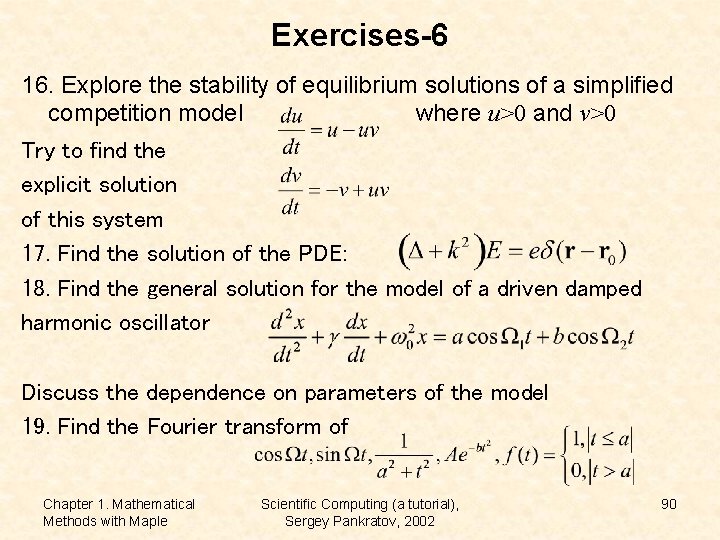
Exercises-6 16. Explore the stability of equilibrium solutions of a simplified competition model where u>0 and v>0 Try to find the explicit solution of this system 17. Find the solution of the PDE: 18. Find the general solution for the model of a driven damped harmonic oscillator Discuss the dependence on parameters of the model 19. Find the Fourier transform of Chapter 1. Mathematical Methods with Maple Scientific Computing (a tutorial), Sergey Pankratov, 2002 90

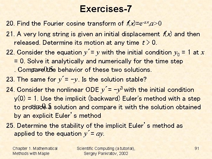
Exercises-7 20. Find the Fourier cosine transform of f(x)=e-ax, a>0 21. A very long string is given an initial displacement f(x) and then released. Determine its motion at any time t > 0. 22. Consider the equation y´= y with the initial condition y 0 = 1 at x = 0. Solve it analytically and numerically for the time step. Compare the behavior of these two solutions. 23. The same for y´= -y. . Is the solution stable? 24. Consider the nonlinear ODE y´= -y 3 with the initial condition y(0) = 1. Use the implicit (backward) Euler's method with a step to produce a solution and compare it with the solution obtained by an explicit Euler’s method 25. Determine the stability of the implicit Euler’s method as applied to the equation y´= ay. Chapter 1. Mathematical Methods with Maple Scientific Computing (a tutorial), Sergey Pankratov, 2002 91

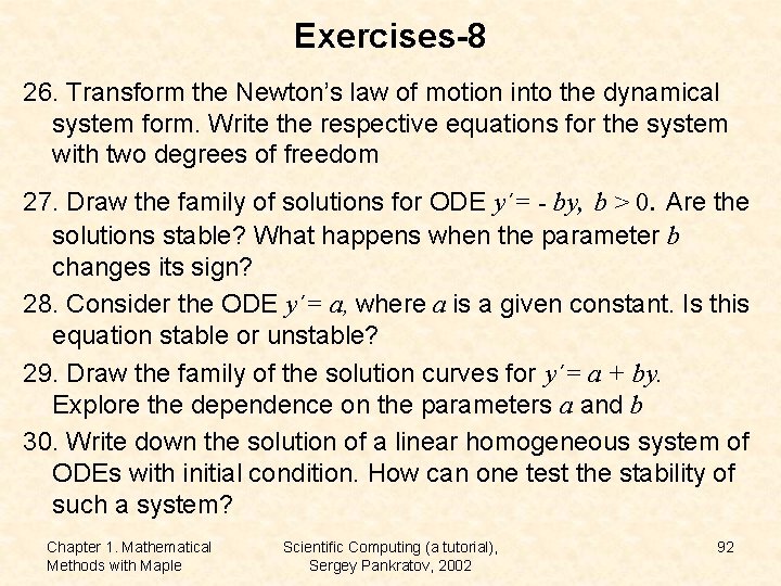
Exercises-8 26. Transform the Newton’s law of motion into the dynamical system form. Write the respective equations for the system with two degrees of freedom 27. Draw the family of solutions for ODE y´= - by, b > 0. Are the solutions stable? What happens when the parameter b changes its sign? 28. Consider the ODE y´= a, where a is a given constant. Is this equation stable or unstable? 29. Draw the family of the solution curves for y´= a + by. Explore the dependence on the parameters a and b 30. Write down the solution of a linear homogeneous system of ODEs with initial condition. How can one test the stability of such a system? Chapter 1. Mathematical Methods with Maple Scientific Computing (a tutorial), Sergey Pankratov, 2002 92