Computing for Scientists Scientific Simulation Sep 27 2010

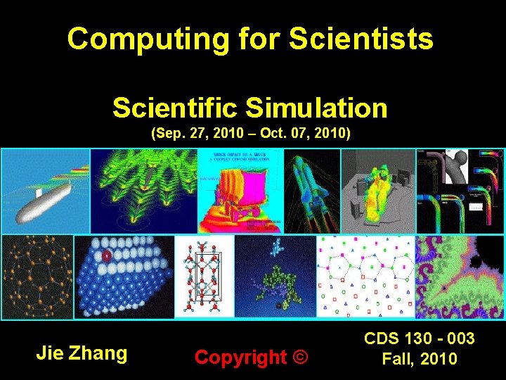
Computing for Scientists Scientific Simulation (Sep. 27, 2010 – Oct. 07, 2010) Jie Zhang Copyright © CDS 130 - 003 Fall, 2010

Motivation • Scientific simulation allows one to reproduce the details of a complex scientific system, e. g. , physical systems, biological systems • It is a new way of scientific research, in additional to traditional experimental and mathematical approaches.

Example Merger of the Milky Way: http: //video. google. com/videoplay? docid=3671579993993423979# The Milky Way and the Andromeda galaxy will likely fall together and merge within a few billion years. In this speculative simulation, the two galaxies flyby one another, exciting tidal tails and bridges and collide on a second pass finally merging after several convulsions. The last remnants of the smashed spirals show up as shells and ripples surrounding a newborn elliptical galaxy.

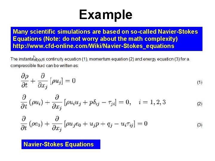
Example Many scientific simulations are based on so-called Navier-Stokes Equations (Note: do not worry about the math complexity) http: //www. cfd-online. com/Wiki/Navier-Stokes_equations Navier-Stokes Equations

Example Cellular Blood Flow: http: //www. youtube. com/watch? v=o 11 NDvr. ZMNs&feature=related The RBCs are modeled as a membrane with hemoglobin inside with a viscosity of 6 c. P. Each RBC membrane is constructed of linear finite element� triangular shells. These shell elements deform due to the fluid-structure interactions with the blood plasma and the hemoglobin.

Objectives 1. Mathematical Models 2. Numerical Methods • Iteration • Differentiation • Integration 3. Verification and Validation

A Pipeline of Models A common way that science gets done 1. Domain specialists (e. g. , biologists) develop a conceptual representation of the system or a scientific model 2. The domain specialists collaborate with mathematicians to develop a mathematical representation, or mathematical model that corresponds to the science model 3. The domain specialists and mathematicians work with computational scientists to implement the equations and explore the results using a computer, that is to develop a computational model of the mathematical model. 4. The computational methods need to be verified, and the results need to be validated.

Mathematical Models (Sep. 29, 2010)

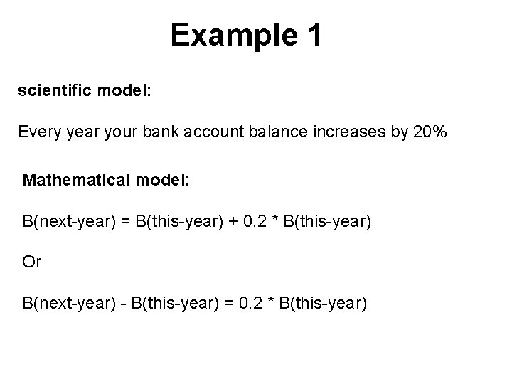
Example 1 scientific model: Every year your bank account balance increases by 20% Mathematical model: B(next-year) = B(this-year) + 0. 2 * B(this-year) Or B(next-year) - B(this-year) = 0. 2 * B(this-year)

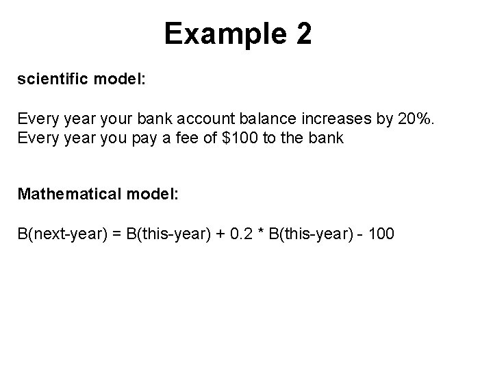
Example 2 scientific model: Every year your bank account balance increases by 20%. Every year you pay a fee of $100 to the bank Mathematical model: B(next-year) = B(this-year) + 0. 2 * B(this-year) - 100

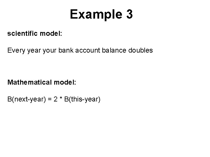
Example 3 scientific model: Every year your bank account balance doubles Mathematical model: B(next-year) = 2 * B(this-year)

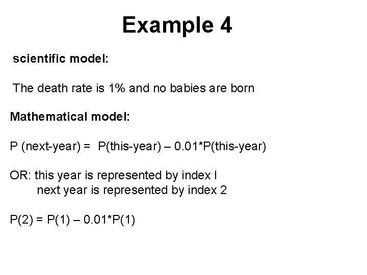
Example 4 scientific model: The death rate is 1% and no babies are born Mathematical model: P (next-year) = P(this-year) – 0. 01*P(this-year) OR: this year is represented by index I next year is represented by index 2 P(2) = P(1) – 0. 01*P(1)

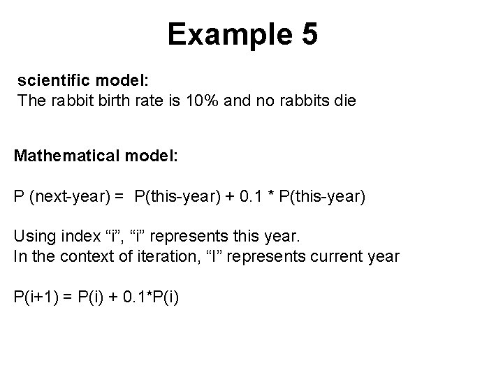
Example 5 scientific model: The rabbit birth rate is 10% and no rabbits die Mathematical model: P (next-year) = P(this-year) + 0. 1 * P(this-year) Using index “i”, “i” represents this year. In the context of iteration, “I” represents current year P(i+1) = P(i) + 0. 1*P(i)

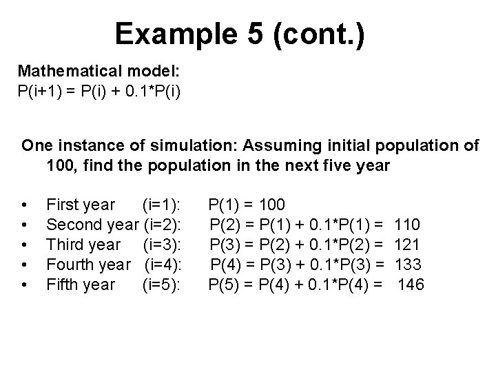
Example 5 (cont. ) Mathematical model: P(i+1) = P(i) + 0. 1*P(i) One instance of simulation: Assuming initial population of 100, find the population in the next five year • • • First year (i=1): Second year (i=2): Third year (i=3): Fourth year (i=4): Fifth year (i=5): P(1) = 100 P(2) = P(1) + 0. 1*P(1) = P(3) = P(2) + 0. 1*P(2) = P(4) = P(3) + 0. 1*P(3) = P(5) = P(4) + 0. 1*P(4) = 110 121 133 146

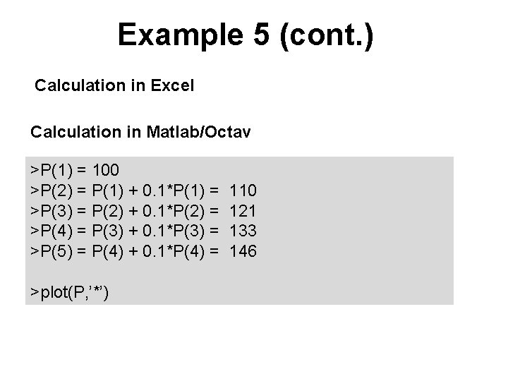
Example 5 (cont. ) Calculation in Excel Calculation in Matlab/Octav >P(1) = 100 >P(2) = P(1) + 0. 1*P(1) = >P(3) = P(2) + 0. 1*P(2) = >P(4) = P(3) + 0. 1*P(3) = >P(5) = P(4) + 0. 1*P(4) = >plot(P, ’*’) 110 121 133 146

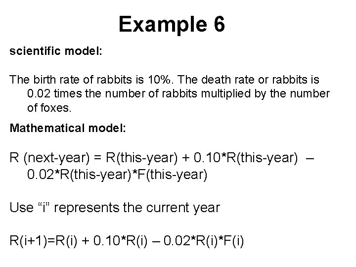
Example 6 scientific model: The birth rate of rabbits is 10%. The death rate or rabbits is 0. 02 times the number of rabbits multiplied by the number of foxes. Mathematical model: R (next-year) = R(this-year) + 0. 10*R(this-year) – 0. 02*R(this-year)*F(this-year) Use “i” represents the current year R(i+1)=R(i) + 0. 10*R(i) – 0. 02*R(i)*F(i)

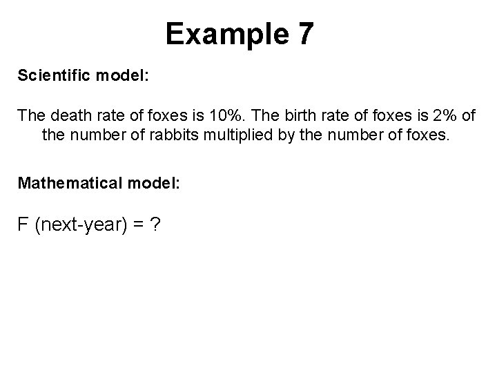
Example 7 Scientific model: The death rate of foxes is 10%. The birth rate of foxes is 2% of the number of rabbits multiplied by the number of foxes. Mathematical model: F (next-year) = ?

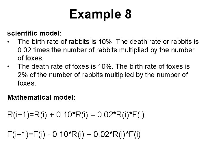
Example 8 scientific model: • The birth rate of rabbits is 10%. The death rate or rabbits is 0. 02 times the number of rabbits multiplied by the number of foxes. • The death rate of foxes is 10%. The birth rate of foxes is 2% of the number of rabbits multiplied by the number of foxes. Mathematical model: R(i+1)=R(i) + 0. 10*R(i) – 0. 02*R(i)*F(i) F(i+1)=F(i) - 0. 10*R(i) + 0. 02*R(i)*F(i)

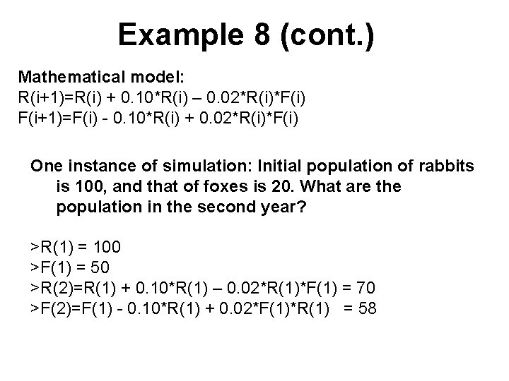
Example 8 (cont. ) Mathematical model: R(i+1)=R(i) + 0. 10*R(i) – 0. 02*R(i)*F(i) F(i+1)=F(i) - 0. 10*R(i) + 0. 02*R(i)*F(i) One instance of simulation: Initial population of rabbits is 100, and that of foxes is 20. What are the population in the second year? >R(1) = 100 >F(1) = 50 >R(2)=R(1) + 0. 10*R(1) – 0. 02*R(1)*F(1) = 70 >F(2)=F(1) - 0. 10*R(1) + 0. 02*F(1)*R(1) = 58

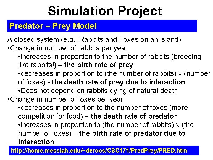
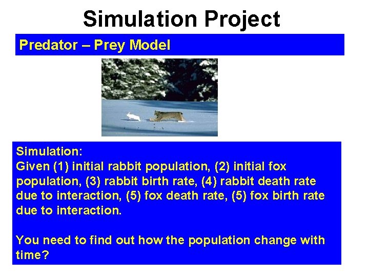
Simulation Project Predator – Prey Model A closed system (e. g. , Rabbits and Foxes on an island) • Change in number of rabbits per year • increases in proportion to the number of rabbits (breeding like rabbits!) – the birth rate of prey • decreases in proportion to (the number of rabbits) x (number of foxes) - the death rate of prey due to interaction • Does not depend on rabbits dying of natural death • Change in number of foxes per year • decreases in proportion to the number of foxes (more competition for food) – the death rate of predator • increases in proportion to (the number of rabbits) x (the number of foxes) – the birth rate of predator due to interaction http: //home. messiah. edu/~deroos/CSC 171/Pred. Prey/PRED. htm

Simulation Project Predator – Prey Model Simulation: Given (1) initial rabbit population, (2) initial fox population, (3) rabbit birth rate, (4) rabbit death rate due to interaction, (5) fox death rate, (5) fox birth rate due to interaction. You need to find out how the population change with time?

Numerical Method - Iteration (Sep. 28, 2010)

To be continued (Sep. 29, 2010)

Verification and Validation (Sep. 29, 2010)