Physics 357457 Spring 2014 Summary The Elementary Particles

Physics 357/457 Spring 2014 Summary §The Elementary Particles § Relativistic Formalism and Lorentz Invariance § Lagrangians and Principle of Least Action § QED and Field Operators § Symmetries and Noether’s Theorem § The Dirac Equation and Spinors § Gauge Fields, Covariant Derivatives and Gauge Bosons § The Standard Model of Elementary Particles § QCD, Gluons and Running Coupling Constants § Cosmology and Particle Physics §Dark Matter, Dark Energy and Inflation

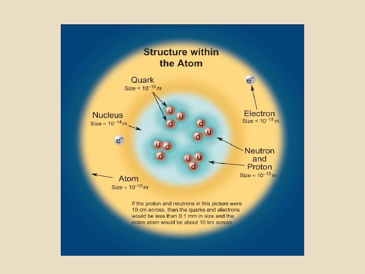
the elementary particles (as far as we know at this time) (u d c s t b) six leptons (e e ) § six quarks § all have spin = ½ they are fermions that’s it!

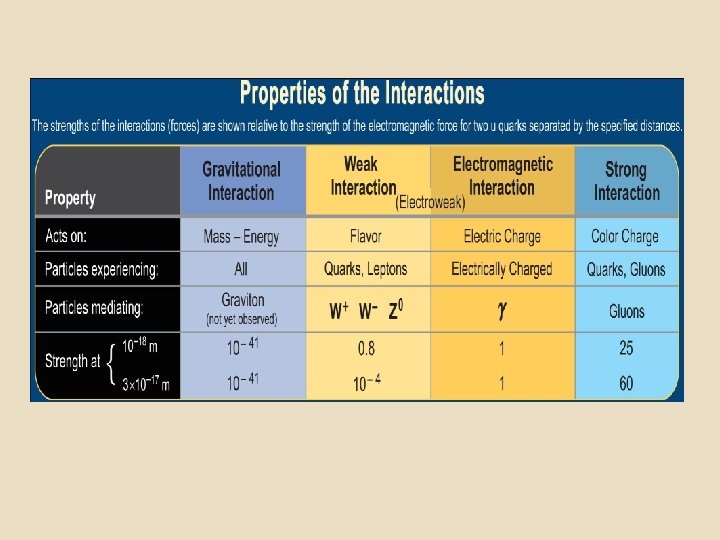
The forces (each force is associated with an exchanged particle) electromagnetic (photon) § weak ( W+ W- Z 0) § strong (8 gluons) § gravitational ( graviton not yet observed) § all have spin = 1 (or 2 for graviton) they are bosons

Review: Special Relativity Einstein’s assumption: the speed of light is independent of the (constant ) velocity, v, of the observer. It forms the basis for special relativity. Speed of light = C = |r 2 – r 1| / (t 2 –t 1) = |r 2’ – r 1’ | / (t 2’ –t 1‘) = |dr/dt| = |dr’/dt’|

4 -dimensional vector component notation • xµ contravariant components • xµ covariant components ( x 0 , x 1 , x 2 , x 3 ) = ( ct, x, y, z ) = (ct, r) µ=0, 1, 2, 3 ( x 0 , x 1 , x 2 , x 3 ) = ( ct, -x, -y, -z ) = (ct, -r) µ=0, 1, 2, 3

Invariant dot products using 4 -component notation contravariant covariant xµ xµ = µ=0, 1, 2, 3 xµ xµ Einstein summation notation (repeated index one up, one down) summation) x µ xµ = (ct)2 -x 2 -y 2 -z 2

Any four vector dot product has the same value in all frames moving with constant velocity w. r. t. each other. Examples: xµ xµ pµ pµ p µ xµ p µ µ µ A µ µ µ

Lorentz Scalars in Momentum Space p = (E/c, px , py , pz ) p p = (E/c)2 – (px)2– (py)2 – (pz)2 is also invariant. In the center of mass of a particle this is equal to (mc 2 /c)2 – (0)2 = m 2 c 2 So, for a particle (in any frame) p p = (E/c)2 – (px)2– (py)2 – (pz)2 = m 2 c 2

Invariant dot products using 4 -component notation µ µ = µ=0, 1, 2, 3 µ µ Einstein summation notation (repeated index summation ) = 2/ (ct)2 - 2 2 = 2/ x 2 + 2/ y 2 + 2/ z 2

Lorentz Invariance • Lorentz invariance of the laws of physics is satisfied if the laws are cast in terms of four-vector dot products! • Four vector dot products are said to be “Lorentz scalars”. • In the relativistic field theories, we must use “Lorentz scalars” to express the interactions.

Standard Model Requires Treatment of Particles as Fields • Hamiltonian, H=E, is not Lorentz invariant. • QM not a relativistic theory. • Lagrangian, T-V, used in particle physics. • Creation and annihilation must be described. • Relativistic Quantum Field theory!

Motivation for Lagrangians and the Law of Least Action

What is a Particle Field? • A good example of a particle field is the electromagnetic field. It can be represented by the field function, A = ( (r, t), A(r, t)). Classically and A are related to E and B. • The zero mass particles, photons, can be created and destroyed and represent the “quantization” of the field.

The wave equations for A and can be put into 4 -vector form: Lorentz gauge! A+ (1/c) / (ct) = 0

Solutions to 1. We have seen how Maxwell’s equations can be cast into a single wave equation for the electromagnetic 4 -vector, Aµ. This Aµ now represents the E and B of the EM field … and something else: the photon! 2. If Aµ is to represent a photon – we want it to be able to represent any photon. That is, we want the most general solution to the equation:

creation operator Spin vector annihilation operator Spin vector This “Fourier expansion” of the photon operator is called “second quantization”. Note that the solution to the wave equation consists of a sum over an infinite number of “photon” creation and annihilation terms. Once the ak± are interpreted as operators, the A becomes an operator.

creation & annihilation operators The procedure by which quantum fields are constructed from individual particles was introduced by Dirac, and is (for historical reasons) known as second quantization. Second quantization refers to expressing a field in terms of creation and annihilation operators, which act on single particle states: |0> = vacuum, no particle |p> = one particle with momentum vector p

From Quantum Mechanics to Lagrangian Densities Just as there is no “derivation” of quantum mechanics from classical mechanics, there is no derivation of relativistic field theory from quantum mechanics. The “route” from one to the other is based on physically reasonable postulates and the imposition of Lorentz invariance and relativistic kinematics. The final “theory” is a model whose survival depends absolutely on its success in producing “numbers” which agree with experiment.

Note that *(r, t) does not represent the probability per unit volume density of the particle being at (r, t).

The “wave equation”:

The field operator for a neutral, spin =0, particle is creates a single particle with momentum p= � k and p 0 = �k 0 at (r, t) Destroys a single particle with momentum p= � k and p 0 = �k 0 at (r, t)

Lagrangians and the Lagrangian Density Recall that, and the Euler-Lagrange equations give F = ma In quantum field theory, the Euler-Lagrange equations give the particle wave function!

This calls for a different kind of “Lagrangian” -- not like the one used in classical or quantum mechanics. So, we have another postulate, defining what is meant by a “Lagrangian” – called a Lagrangian d/dt in the classical theory density.

Summary for neutral (Q=0) scalar (spin = 0) particle, , with mass, m. Lagrangian density wave equation field operator

Particles with Charge: two fields , and * From the Lagrangian density and the Euler-Lagrange equation we can derive the wave equation

creates positively charged particle with momentum p= � k and p 0 = �k 0 at (r, t) destroys negatively charged particle with momentum p= � k and p 0 = �k 0 at (r, t) creates negatively charged particle with momentum p= � k and p 0 = �k 0 at (r, t)

Gauge Invariance and Conserved Quantities “Noether's theorem” was proven by German mathematician, Emmy Noether in 1916 and published in 1918. Noether's theorem has become a fundamental tool of quantum field theory – and has been called "one of the most important mathematical theorems ever proved in guiding the development of modern physics". Amalie Emmy Noether 1882 -1935

An astounding result: we can vary the (complex) phase of the field operator, , everywhere in space by any continuous amount and not affect the “laws of physics” (that is the L) which govern the system! Note that everywhere in space the phase changes by the same . This is called a global symmetry. ’ Remember Emmy Noether!

With the help of Emmy Noether, we can prove that charge is conserved!

Deriving the conserved current and the conserved charge: Euler-Lagrange equation conserved current But our Lagrangian density also contains a *, so we obtain additional terms like the above, with replaced by *. In each case the Euler –Lagrange equations are satisfied. So, the remaining term is as follows: = 0 gives charge operator!

This is how transforms: Now we evaluate . The great advantage of being a continuous constant is that there an infinite number of very small which carry with them all the physics of the “continuity”. That is, with no loss of rigor we can assume is small!

The value of the charge is calculated from: the charge operator. integrate over time S 0(t) outgoing particle integrate over all space One obtains a number! p p incoming outgoing incoming particle

Calculation of Charge

Note Dirac delta function in k and p ‘

The time disappears! Q is time independent. The integration over k’ is done with the Dirac delta function from the d 3 x integration. The remaining integration over k will be done with the Dirac delta functions from the commutation relations. Note: + and/or – must be together.

Message: calculating charge is a lot of work -- but can be done!

Fermions and the Dirac Equation In 1928 Dirac proposed the following form for the electron wave equation: 4 -row column matrix 4 x 4 unit matrix The four µ matrices form a Lorentz 4 -vector, with components, µ. That is, they transform like a 4 -vector under Lorentz transformations between moving frames. Each µ is a 4 x 4 matrix.

The Dirac equation in full matrix form 0 1 2 3 spin dependence space-time dependence

Spinors for the particle with p along z direction p along z and spin = +1/2 p along z and spin = -1/2

Field operator for the spin ½ fermion Spinor for antiparticle with momentum p and spin s Creates antiparticle with momentum p and spin s Note: pµ pµ = m 2 c 2

Lagrangian Density for Spin 1/2 Fermions Comments: 1. This Lagrangian density is used for all the quarks and leptons – only the masses will be different! 2. The Euler Lagrange equations, when applied to this Lagrangian density, give the Dirac Equation! 3. Note that L is a Lorentz scalar.

Lagrangian Density for Spin 1/2 Quarks and Leptons Now we are ready to talk about the gauge invariance that leads to the Standard Model and all its interactions. Remember a “gauge invariance” is the invariance of the above Lagrangian under transformations like e i . The physics is in the -- which can be a matrix operator and depend on x, y, z and t.

Local Gauge Invariance and Existence of the Gauge Particles 1. Gauge transformations are like “rotations” 2. How do functions transform under “rotations”? 3. How can we generalize to rotations in “strange” spaces (spin space, , flavor space, color space)? 4. How are Lagrangians made invariant under these “rotations”? (Lagrangians “laws of physics” for particles interactions. ) 5. Invariance of L requires the existence of the gauge boson!

This is how the function transforms when x x + x

momentum operator x component momentum operator

angular momentum operator The angular momentum operator, generates rotations in x, y, z space!

Gauge transformations are like the “rotations” we have just been considering Real function of space and time one has to find a Lagrangian which is invariant under this transformation. can be an operator -- as we have just seen.

How are Lagrangians made invariant under these “rotations”? It won’t work!

Constructing a gauge invariant Lagrangian: 1. Begin with the “old Lagrangian”: called the “covariant derivative” 2. Replace Aµ is the gauge boson (exchange particle) field! 3. “old” Lagrangian the interaction term.

Showing L is invariant transformed L transformed A µ = Aµ - (1/e) transformed A Maxwell’s equations are invariant under this!

Summary of Local gauge symmetry Real function of space and time covariant derivative The final invariant L is given by:

The correct, invariant Lagrangian density, includes the interaction between the electron (fermion) and the photon (the gauge particle). free electron Lagrangian interaction Lagrangian If the coupling, e, is turned off, L reverts to the free electron L. This use of the covariant derivative will be applied to all the interaction terms of the Standard Model.

Comments: 1. There is no difference between changing the phase of the field operator of the fermion (by (r, t) at every point in space) and the effects of a gauge transformation [ -(1/e) µ (r, t) ] on the photon field! 2. Maxwell’s equations are invariant under A µ - (1/e) µ (r, t) -- and, in particular, the gauge transformation has no effect on the free photon. 3. It is only because (r, t) depends on r and t that the above is possible. This is called a local gauge transformation. 4. Note that a global gauge transformation would require that is a constant!

Lecture 10: Standard Model Lagrangian The Standard Model Lagrangian is obtained by imposing three local gauge invariances on the quark and lepton field operators: symmetry: U(1) “QED-like” SU(2) weak SU(3) color gauge boson neutral gauge boson 3 heavy vector bosons 8 gluons This gives rise to 1 + 3 + 8 spin = 1 force carrying gauge particles.

SU(2) and SU(n) dot product Pauli spin matrix functions of x, y, z, t The are called the generators of the group. n = 2 3 components 3 gauge particles

SU(2): rotations in Flavor Space “rotated” flavor state original flavor state These are the Pauli spin matrices, 1 2 3 local depends on x, y, z, and t.

Flavor Space Flavor space is used to describe an intrinsic property of a particle. While this is not (x, y, z, t) space we can use the same mathematical tools to describe it. Flavor space can be thought of as a three dimensional space. The particle eigenstates we know about (quarks and leptons) are “doublets” with flavor up or down – along the “ 3” axis.

Summary: QED local gauge symmetry Real function of space and time covariant derivative The final invariant L is given by:

SU(2) local gauge symmetry generator of SU(2) rotations in flavor space! covariant derivative The final invariant L is given by: coupling constant generators of SU(2) interaction term

Rotations (on quark states) in color space: SU(3) The quarks are assumed to carry an additional property called color. So, for the down quark, d, we have the “down quark color triplet”: quark field operators red = d red green = d green blue = d blue There is a color triplet for each quark: u, d, c, s, t, and b, but, for now we won’t need the t and b.

A general “rotation” in color space can be written as a local, (non-abelian) SU(3) gauge transformation local generators of SU(3) red green blue a = 1, 2, 3, … 8 Since the a don’t commute, the SU(3) gauge transformations are non-abelian.

The generators of SU(3): eight 3 x 3 a matrices (a = 1, 2, 3… 8) 1 = 2 = 3 = 4 = 5 = 6 = 7 = 8 = (n 2 – 1) = 32 - 1 = 8 generators All 3 x 3 matrix elements of SU(3) can be written as a linear combination of these 8 a plus the identity matrix.

[ 11, 22] the a don’t commute = 2 i f 1123 3 3 f 123 = 1 = - f 213 = f 231 Likewise one can show: (for the graduate students) fabc = -fbac = fbca f 458 = f 678 = 3 /2, f 147 = f 516 = f 246 = f 257 = f 345 = f 637 = ½ … all the rest = 0.

SU(3) gauge invariance in the Standard Model generators of SU(3) The invariant Lagrangian density is given by: interaction term

The Lagrangian density with the U(1), SU(2) and SU(3) gauge particle interactions Y neutral vector boson heavy vectors bosons (W , W 3) 8 gluons

Standard Model Lagrangian with Electro-Weak Unification The Standard Model assumes that the mass of the neutrino is zero and that it is “left handed” -- travelling with its spin pointing opposite to its direction of motion. Since in this case there would be no “right handed” neutrino, the “flavor” partner of the neutrino must be a “left handed” electron. This changes the structure of the Standard Model Lagrangian – which is assumed to treat only left handed flavor doublets.

These are the only spinors allowed for a zero mass neutrino! positive helicity negative helicity The neutrino, if it has a zero mass can only have its spin pointing along (or opposite to) it’s momentum.

Non-conservation of parity: Wu 1957

Each term in the SM Lagrangian density containing quarks and the leptons can be rewritten using the following expression. For the neutrinos, however, only the left handed term exists. In the following slide we use the notation d R = d. R

The following is the interaction Lagrangian density for the first generation of particles with the left and right handed parts shown explicitly. B B B W 1 W 2 + B W 3 sum over a = 1, 2, … 8 a Ga

Weinberg’s decomposition of the B and W: W = Weinberg angle -- to be determined experimentally! sin 2 W 0. 23

Next steps: rewriting interaction Lagrangian density so that interactions with the photon are identified. 1. 2. 3. The neutrino has zero charge and can’t interact with the photon.

After substituting the expressions for B and W 0 (which takes some work), one can identify factors which equal e, the electronic charge, or the up quark charge, etc. This permits one to find relationships between sin W , cos W , e, g 2 and g 1. One finds that: Also one defines: g 2 = e / sin W g 1 = e / cos W T 3 f YL = -1 YR = 2 Y L = + 1/2 for the u. L = - 1/2 for the d. L = 0 for u. R = 0 for d. R

The Standard Model Interaction Lagrangian for the 1 st generation (E & M) QED interactions weak neutral current interactions + weak flavor changing interactions + QCD color interactions

The U(1) and SU(2) interaction terms g 2 = e / sin W e A (E & M) QED interactions g 2 Z + Z weak neutral current interactions g 2 W+ weak flavor changing interactions W-

The following values for the constants gives the correct charge for all the particles.

Weak neutral current interactions Z 0

Weak charged flavor changing interactions quarks leptons g 2

Quantum Chromodynamics (QCD): color forces Only non-zero components of contribute.

To find the final form of the QCD terms, we rewrite the above sum, collecting similar quark “color” combinations.

The QCD interaction Lagrangian density

Note that there are only 8 possibilities: grrg-g ggb- The red, anti-green gluon The green, anti-blue gluon

The gluon forces hold the proton together proton At any time the proton is color neutral. That is, it contains one red, one blue and one green quark.

beta decay u u d d d u W- neutron W doesn’t see color proton

W production from p p- d u u -d -u -u W+ ppp--

The nuclear force u n u d d d u u p W- p u d d d u u Note that W- d + u- = - In older theories, one would consider rather the exchange of a - between the n and p. n

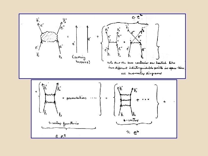
Cross sections and Feynman diagrams everything happens here transition probability amplitude must sum over all possible Feynman diagram amplitudes with the same initial and final states.

Feynman rules applied to a 2 -vertex electron positron scattering diagram Note that each vertex is generated by the interaction Lagrangian density. time spin metric tensor Mfi = left vertex function coupling constant – one for each vertex right vertex function propagator The next steps are to do the sum over and carry out the matrix multiplications. Note that is a 4 x 4 matrix and the spinors are 4 -component vectors. The result is a a function of the momenta only, and the four spin (helicity) states.

Confinement of quarks free quark terms free gluon terms quark- gluon interactions The free gluon terms have products of 2, 3 and 4 gluon field operators. These terms lead to the interaction of gluons with other gluons.

G normal free gluon term Nf= # flavors G Note sign 3 -gluon vertex Nc= # colors Nf quark loop Nc gluon loop

momentum squared of exchanged gluon Nf Nc M 2 quark Nf Nc -7 In QED one has no terms corresponding to the number of colors (the 3 -gluon) vertex. This term aslo has a negative sign.

Quark confinement arises from the increasing strength of the interaction at long range. At short range the gluon force is weak; at long range it is strong. This confinement arises from the SU(3) symmetry – with it’s non-commuting (non-abelian) group elements. This non-commuting property generates terms in the Lagrangian density which produce 3 -gluon vertices – and gluon loops in the exchanged gluon “propagator”.

Grand Unified Theory, Running Coupling Constants and the Story of our Universe These next theories are in a less rigorous state and we shall talk about them, keeping in mind that they are at the ‘”edge” of what is understood today. Nevertheless, they represent a qualitative view of our universe, from the perspective of particle physics and cosmology. GUT -- Grand Unified Theories – symmetry between quarks and leptons; decay of the proton. Running coupling constants: it’s possible that at one time in the development of the universe all the forces had the same strength The Early Universe: a big bang, cooling and expanding, phase transitions and broken symmetries

We have incorporated into the Lagrangian density invariance under rotations in U(1)XSU(2)flavor space and SU(3)color space, but these were not really unified. That is, the gauge bosons, (photon, W, and Z, and gluons) were not manifestations of the same force field. If one were to “unify” these fields, how might it occur? The attempts to do so are called Grand Unified Theories. Grand Unified Theory (GUT) GUT includes invariance under U(1) X SU(2)flavor space and SU(3)color and invariance under the following transformations: quarks leptons quarks

Grand Unified Theory - SU(5) Georgii & Glashow, Phys. Rev Lett. 32, 438 (1974). d red dgreen d blue e- rgb L SU(5) gau Quarks & leptons in same multiplet ; mx 1015 Ge. V 8 gluons 24 Gauge bosons (W 0+B) W- Left handed Gauge invariance For symmetry under SU(5), the L SU(5) W+ (W 0 +B) is invariant under e-i (x, y, t) x and y particles must be massless!

SU(5) generators and covariant derivative The 52 -1 = 24 generators of SU(5) are the i do not commute. SU(5) is a non-abelian local gauge theory. 24 components: i(x, y, t) = 5 x 5 matrices which i(x, y, t) has all real, continuous functions D = - i g 5/2 j. Xi j=1, 24 where Xi = the 24 gauge bosons This includes the Standard Model covariant derivative (couplings are different). Predictions: a) qup = 2/3 ; qd = -1/3 b) sin 2 W -. 23 c) the proton decays! > 1034 years d) baryon number not conserved e) only one coupling constant, g 5 (g 1, g 2, and g 3, are related) So far, there is no evidence that the proton decays. But note that the lifetime of the universe is 14 billion years. The probability of detecting a decaying proton depends a large sample of protons!

- X + = 1, 2, 3 quark to lepton, no color change 3 -color vertex Q = - 4/3 Y - = 1, 2, 3 quark to lepton, no color change 3 -color vertex Q= - 1/3 + Hermitian Conjugate (contains X + and Y + terms) Charge conjugation operator T transpose Note: one coupling constant, g 5

charge X-4/3 red e+ dred e+

Decay of proton in SU(5) d red - u green d red u blue proton - green Xred X+ red 3 -color vertex anti-up 0 blue e+ X +red green blue

SUPER SYMMETRIC (SUSY) THEORIES: SUSYs contain invariance of the Lagrangian density under operations which change bosons (spin = 01, 2, . . ) fermions (spin = ½, 3/2 …). SUSY unifies E&M, weak, strong (SU(3) and gravity fields. usually includes invariance under local transformations http: //www. pha. jhu. edu/~gbruhn/Intro. SUSY. html Supergravity

Supersymmetric String Theories Elementary particles are one-dimensional strings: open strings closed strings or . no free parameters L = 2 r L = 10 -33 cm. = Planck Length Mplanck 1019 Ge. V/c 2 See Schwarz, Physics Today, November 1987, p. 33 “Superstrings” The Planck Mass is approximately that mass whose gravitational potential is the same strength as the strong QCD force at r 10 -15 cm. An alternate definition is the mass of the Planck Particle, a hypothetical miniscule black hole whose Schwarzchild radius is equal to the Planck Length.

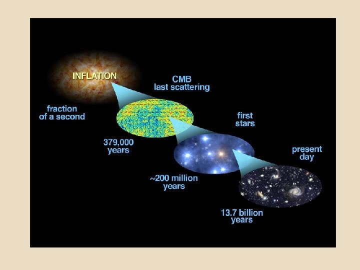
Particle Physics and the Development of the Universe Very early universe All ideas concerning the very early universe are speculative. As of early today, no accelerator experiments probe energies of sufficient magnitude to provide any experimental insight into the behavior of matter at the energy levels that prevailed during this period. Planck epoch Up to 10 – 43 seconds after the Big Bang At the energy levels that prevailed during the Planck epoch the four fundamental forces— electromagnetism U(1) , gravitation, weak SU(2), and the strong SU(3) color — are assumed to all have the same strength, and “unified” in one fundamental force. Little is known about this epoch. Theories of supergravity/ supersymmetry, such as string theory, are candidates for describing this era.

Grand unification epoch: GUT Between 10– 43 seconds and 10– 36 seconds after the Big Bang The universe expands and cools from the Planck epoch. After about 10– 43 seconds the gravitational interactions are no longer unified with the electromagnetic U(1) , weak SU(2), and the strong SU(3) color interactions. Supersymmetry/Supergravity symmetires are roken. After 10– 43 seconds the universe enters the Grand Unified Theory (GUT) epoch. A candidate for GUT is SU(5) symmetry. In this realm the proton can decay, quarks are changed into leptons and all the gauge particles (X, Y, W, Z, gluons and photons), quarks and leptons are massless. The strong, weak and electromagnetic fields are unified.

Running Coupling Constants Electro weak unification Electro. Weak Symmetry breaking Planck region Supersymmetry SU(3) GUT electroweak Ge. V

Inflation and Spontaneous Symmetry Breaking. At about 10– 36 seconds and an average thermal energy k. T 1015 Ge. V, a phase transition is believed to have taken place. In this phase transition, the vacuum state undergoes spontaneous symmetry breaking. Spontaneous symmetry breaking: Consider a system in which all the spins can be up, or all can be down – with each configuration having the same energy. There is perfect symmetry between the two states and one could, in theory, transform the system from one state to the other without altering the energy. But, when the system actually selects a configuration where all the spins are up, the symmetry is “spontaneously” broken.

Higgs Mechanism When the phase transition takes place the vacuum state transforms into a Higgs particle (with mass) and so-called Goldstone bosons with no mass. The Goldstone bosons “give up” their mass to the gauge particles (X and Y gain masses 1015 Ge. V). The Higgs keeps its mass ( thermal energy of the universe, k. T 1015 Ge. V). This Higgs particle has too large a mass to be seen in accelerators. What causes the inflation? The universe “falls into” a low energy state, oscillates about the minimum (giving rise to the masses) and then expands rapidly. When the phase transition takes place, latent heat (energy) is released. The X and Y decay into ordinary particles, giving off energy. It is this rapid expansion that results in the inflation and gives rise to the “flat” and homogeneous universe we observe today. The expansion is exponential in time.

Schematic of Inflation 1019 T (Ge. V/k) R(t) m R t 2/3 R t 1/2 T t-1/2 R e. Ht 1014 T t-1/2 R t 1/2 T t-2/3 T=2. 7 K 10 -13 10 -43 10 -34 10 -31 time (sec) 10

Electroweak epoch Between 10– 36 seconds and 10– 12 seconds after the Big Bang The SU(3) color force is no longer unified with the U(1)x SU(2) weak force. The only surviving symmetries are: SU(3) separately, and U(1)X SU(2). The W and Z are massless. A second phase transition takes place at about 10– 12 seconds at k. T = 100 Ge. V. In this phase transition, a second Higgs particle is generated with mass close to 100 Ge. V; the Goldstone bosons give up their mass to the W, Z and the particles (quarks and leptons). It is the search for this second Higgs particle that is taking place in the particle accelerators at the present time.

After the Big Bang: the first 10 -6 Seconds Planck Era SUSY Supergravity inflation gravity. X, Y take decouples on mass GUT W , Z 0 take on mass SU(2) x U(1) symmetry . all forces unified bosons fermions quarks leptons all particles massless .

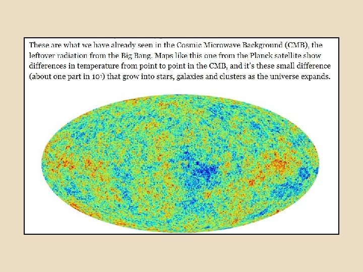
. W , Z 0 take on mass COBE data. 2. 7 K Standard Model 100 Gev . . . only gluons and photons are massless n, p formed nuclei formed atoms formed

Dark Matter • cannot be seen directly with telescopes; it neither emits nor absorbs light; • estimated to constitute 84. 5% of the total matter in the universe – and 26. 8% of the total mass/energy of the universe; • its existence is inferred from gravitational effects on visible matter and gravitational lensing of background radiation;

Rotational curves for a typical galaxy indicate that the mass of the galaxy is not concentrated in its center. Our own galaxy is predicted to have a spherical halo of dark matter.

Visualization of dark matter halo for spiral galaxy

Candidates for nonbaryonic dark matter • Axions (0 spin, 0 charge, small mass, Goldstone bosons) • Supersymmetric particles (partners in SUZY) – not been seen yet • Neutrinos (small fraction ) • Weakly interacting massive particles. . so far none have been detected.

Dark Energy • The size and the smoothness of the Universe can be explained by very rapid expansion—inflation. • However, there is not enough observable matter to generate stars or galaxies. The force of gravity from observable matter is too weak. This is one of a number of reasons we need dark matter. • Finally, to explain the acceleration of the expansion of the Universe, we need dark energy; ideally, that would explain both early inflation and today's inflation.

Begin with the metric tensor for the 4 dimensional space: General Relativity. ds is measure of distance between two points scale factor

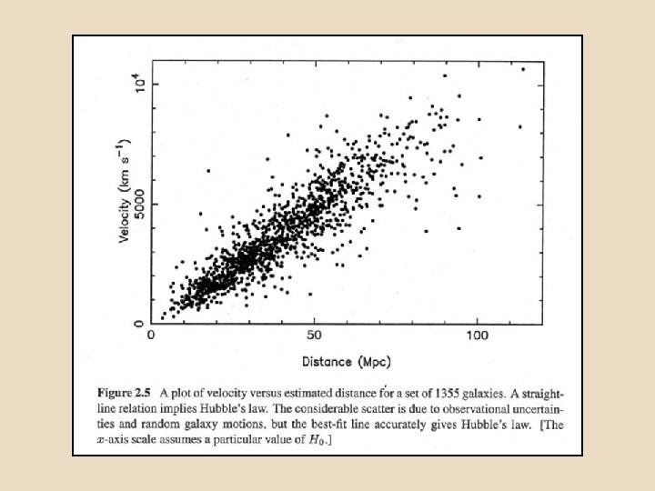
Rather than the relativistic red shift, the Cosmological red shift is now used in interpreting the Hubble constant: 1 + z = R(tnow)/R(tthen) 1 + z = observed/ emitted z = ( observed - emitted)/ emitted Hubble’s Law: v=Hd v = recessional speed H = Hubble’s constant d = distance

Acceleration of the expansion of the observable universe is at this point too small to affect the “measured” value of the Hubble constant. But one can see from the following expression that an increase in H must follow from a term not yet included in the equation of state. missing terms – due to dark energy?

Einstein’s Equations and Hubble Law Derivation … use Noether’s theorem. S=0 Einstein ‘s equations

The = = 0 component of Einstein’s equations gives Hubble’s Law: https: //www. youtube. com/watch? v=EIp. Ez. Zqkd 9 c d. E = -pd. V

Some comments on Inflation: potential form. possible tunneling long slow “roll” into minimum Energetic coherent oscillations about minimum steep asymmetric rise absolute minimum

Difference between polarization characteristic of density fluctuations and gravitational waves:

On March 17, 2014 scientists announced the first direct detection of the cosmic inflation behind the rapid expansion of the universe just a tiny fraction of a second after the Big Bang 13. 8 billion years ago. A key piece of the discovery is the evidence of gravitational waves, a long-sought cosmic phenomenon that has eluded astronomers until now. https: //www. youtube. com/watch? v=PCx. OEyyzmv. Q

With classical Newtonian mechanics and electrodynamics we probed large scale phenomena in our solar system. We looked outward to study the stars and galaxies, and the expanding space of our observable universe. Atomic scale theories of quantum mechanical phenomena and relativistic formalisms generated technology which made these studies possible. Probing deeper into nuclei, quarks, leptons, symmetry generated gauge bosons, and general relativity we are at the brink of understanding the story of our universe itself. And we have learned of the far-reaching implications of symmetry