CS 1699 Deep Learning Neural Network Training Part

![“Xavier initialization” [Glorot et al. , 2010] Reasonable initialization. (Mathematical derivation assumes linear activations) “Xavier initialization” [Glorot et al. , 2010] Reasonable initialization. (Mathematical derivation assumes linear activations)](https://slidetodoc.com/presentation_image_h2/9895368f71e9327388947d823a2357bc/image-9.jpg)
![Activation Functions - Squashes numbers to range [0, 1] - Historically popular since they Activation Functions - Squashes numbers to range [0, 1] - Historically popular since they](https://slidetodoc.com/presentation_image_h2/9895368f71e9327388947d823a2357bc/image-11.jpg)
![Activation Functions - Squashes numbers to range [0, 1] - Historically popular since they Activation Functions - Squashes numbers to range [0, 1] - Historically popular since they](https://slidetodoc.com/presentation_image_h2/9895368f71e9327388947d823a2357bc/image-12.jpg)
![Activation Functions - Squashes numbers to range [0, 1] - Historically popular since they Activation Functions - Squashes numbers to range [0, 1] - Historically popular since they](https://slidetodoc.com/presentation_image_h2/9895368f71e9327388947d823a2357bc/image-14.jpg)
![Activation Functions - Squashes numbers to range [0, 1] - Historically popular since they Activation Functions - Squashes numbers to range [0, 1] - Historically popular since they](https://slidetodoc.com/presentation_image_h2/9895368f71e9327388947d823a2357bc/image-15.jpg)
![Activation Functions - Squashes numbers to range [-1, 1] - zero centered (nice) - Activation Functions - Squashes numbers to range [-1, 1] - zero centered (nice) -](https://slidetodoc.com/presentation_image_h2/9895368f71e9327388947d823a2357bc/image-16.jpg)
![[Mass et al. , 2013] [He et al. , 2015] Activation Functions - Does [Mass et al. , 2013] [He et al. , 2015] Activation Functions - Does](https://slidetodoc.com/presentation_image_h2/9895368f71e9327388947d823a2357bc/image-21.jpg)
![[Mass et al. , 2013] [He et al. , 2015] Activation Functions - Does [Mass et al. , 2013] [He et al. , 2015] Activation Functions - Does](https://slidetodoc.com/presentation_image_h2/9895368f71e9327388947d823a2357bc/image-22.jpg)
![[Clevert et al. , 2015] Activation Functions Exponential Linear Units (ELU) - All benefits [Clevert et al. , 2015] Activation Functions Exponential Linear Units (ELU) - All benefits](https://slidetodoc.com/presentation_image_h2/9895368f71e9327388947d823a2357bc/image-23.jpg)
![[Goodfellow et al. , 2013] Maxout “Neuron” - Does not have the basic form [Goodfellow et al. , 2013] Maxout “Neuron” - Does not have the basic form](https://slidetodoc.com/presentation_image_h2/9895368f71e9327388947d823a2357bc/image-24.jpg)
![Batch Normalization [Ioffe and Szegedy, 2015] “you want zero-mean unit-variance activations? just make them Batch Normalization [Ioffe and Szegedy, 2015] “you want zero-mean unit-variance activations? just make them](https://slidetodoc.com/presentation_image_h2/9895368f71e9327388947d823a2357bc/image-26.jpg)
![Batch Normalization [Ioffe and Szegedy, 2015] “you want zero-mean unit-variance activations? just make them Batch Normalization [Ioffe and Szegedy, 2015] “you want zero-mean unit-variance activations? just make them](https://slidetodoc.com/presentation_image_h2/9895368f71e9327388947d823a2357bc/image-27.jpg)
![Batch Normalization [Ioffe and Szegedy, 2015] Normalize: Note, the network can learn: And then Batch Normalization [Ioffe and Szegedy, 2015] Normalize: Note, the network can learn: And then](https://slidetodoc.com/presentation_image_h2/9895368f71e9327388947d823a2357bc/image-28.jpg)
![Batch Normalization [Ioffe and Szegedy, 2015] - Improves gradient flow through the network - Batch Normalization [Ioffe and Szegedy, 2015] - Improves gradient flow through the network -](https://slidetodoc.com/presentation_image_h2/9895368f71e9327388947d823a2357bc/image-29.jpg)
![Batch Normalization [Ioffe and Szegedy, 2015] Note: at test time Batch. Norm layer functions Batch Normalization [Ioffe and Szegedy, 2015] Note: at test time Batch. Norm layer functions](https://slidetodoc.com/presentation_image_h2/9895368f71e9327388947d823a2357bc/image-30.jpg)




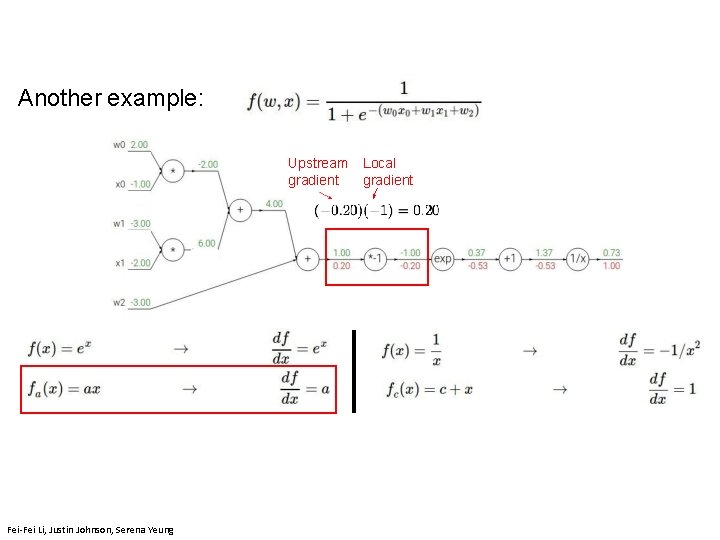
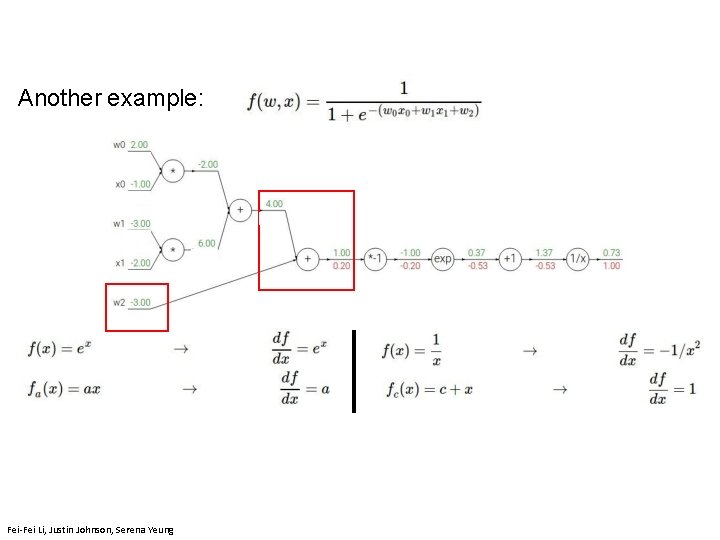
![Another example: [upstream gradient] x [local gradient] [0. 2] x [1] = 0. 2 Another example: [upstream gradient] x [local gradient] [0. 2] x [1] = 0. 2](https://slidetodoc.com/presentation_image_h2/9895368f71e9327388947d823a2357bc/image-151.jpg)
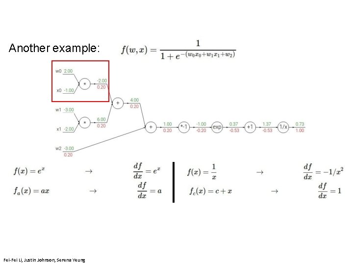
![Another example: [upstream gradient] x [local gradient] x 0: [0. 2] x [2] = Another example: [upstream gradient] x [local gradient] x 0: [0. 2] x [2] =](https://slidetodoc.com/presentation_image_h2/9895368f71e9327388947d823a2357bc/image-153.jpg)
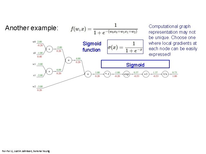
![Backprop with Vectors 4 D input x: [ 1 ] [ -2 ] [ Backprop with Vectors 4 D input x: [ 1 ] [ -2 ] [](https://slidetodoc.com/presentation_image_h2/9895368f71e9327388947d823a2357bc/image-178.jpg)
![Backprop with Vectors 4 D input x: [ 1 ] [ -2 ] [ Backprop with Vectors 4 D input x: [ 1 ] [ -2 ] [](https://slidetodoc.com/presentation_image_h2/9895368f71e9327388947d823a2357bc/image-179.jpg)
![Backprop with Vectors 4 D input x: [ 1 ] [ -2 ] [ Backprop with Vectors 4 D input x: [ 1 ] [ -2 ] [](https://slidetodoc.com/presentation_image_h2/9895368f71e9327388947d823a2357bc/image-180.jpg)
![Backprop with Vectors 4 D input x: [ 1 ] [ -2 ] [ Backprop with Vectors 4 D input x: [ 1 ] [ -2 ] [](https://slidetodoc.com/presentation_image_h2/9895368f71e9327388947d823a2357bc/image-181.jpg)
![Backprop with Vectors 4 D input x: [ 1 ] [ -2 ] [ Backprop with Vectors 4 D input x: [ 1 ] [ -2 ] [](https://slidetodoc.com/presentation_image_h2/9895368f71e9327388947d823a2357bc/image-182.jpg)
![Backprop with Matrices (or Tensors) [Dx×Mx] “local gradients” [Dx×Mx] [Dy×My] d. L/dx always has Backprop with Matrices (or Tensors) [Dx×Mx] “local gradients” [Dx×Mx] [Dy×My] d. L/dx always has](https://slidetodoc.com/presentation_image_h2/9895368f71e9327388947d823a2357bc/image-184.jpg)
- Slides: 196

CS 1699: Deep Learning Neural Network Training (Part 2) Prof. Adriana Kovashka University of Pittsburgh February 4, 2020

Plan for this lecture • Tricks of the trade • Convergence of gradient descent – How long will it take? – Will it work at all? • Different optimization strategies – Alternatives to SGD – Learning rates – Choosing hyperparameters • How to do the computation – Computation graphs – Vector notation (Jacobians)

Tricks of the trade

Practical matters • Getting started: Preprocessing, initialization, normalization, choosing activation functions • Improving performance and dealing with sparse data: regularization, augmentation, transfer • Hardware and software

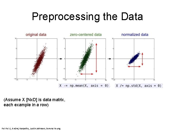
Preprocessing the Data Fei-Fei Li & Justin Johnson & Serena Yeung Lecture 6 - 5 April 19, 2018 (Assume X [Nx. D] is data matrix, each example in a row) Fei-Fei Li & Justin Johnson & Serena Yeung Lecture 6 - April 19, 2018 Fei-Fei Li, Andrej Karpathy, Justin Johnson, Serena Yeung

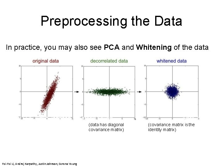
Preprocessing the Data In practice, you may also see PCA and Whitening of the data April 19, 2018 Fei-Fei Li & Justin Johnson & Serena Yeung (data has diagonal covariance matrix) Fei-Fei Li & Justin Johnson & Serena Yeung Fei-Fei Li, Andrej Karpathy, Justin Johnson, Serena Yeung (covariance matrix is the identity matrix) Lecture 6 - 39 April 19, 2018

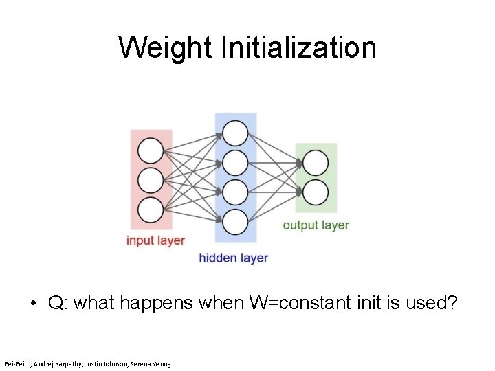
Weight Initialization • Q: what happens when W=constant init is used? April 19, 2018 Fei-Fei Li, Andrej Karpathy, Justin Johnson, Serena Yeung

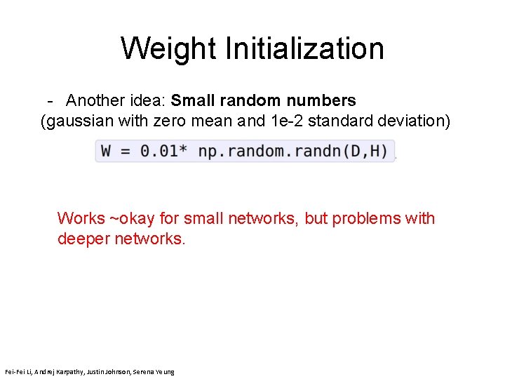
Weight Initialization - Another idea: Small random numbers (gaussian with zero mean and 1 e-2 standard deviation) Works ~okay for small networks, but problems with deeper networks. Fei-Fei Li & Justin Johnson & Serena Yeung Lecture 6 - 8 April 19, 2018 Fei-Fei Li & Justin Johnson & Serena Yeung Lecture 6 - April 19, 2018 Fei-Fei Li, Andrej Karpathy, Justin Johnson, Serena Yeung
![Xavier initialization Glorot et al 2010 Reasonable initialization Mathematical derivation assumes linear activations “Xavier initialization” [Glorot et al. , 2010] Reasonable initialization. (Mathematical derivation assumes linear activations)](https://slidetodoc.com/presentation_image_h2/9895368f71e9327388947d823a2357bc/image-9.jpg)
“Xavier initialization” [Glorot et al. , 2010] Reasonable initialization. (Mathematical derivation assumes linear activations) April 19, 2018 Fei-Fei Li & Justin Johnson & Serena Yeung Fei-Fei Li, Andrej Karpathy, Justin Johnson, Serena Yeung Lecture 6 - April 19, 2018

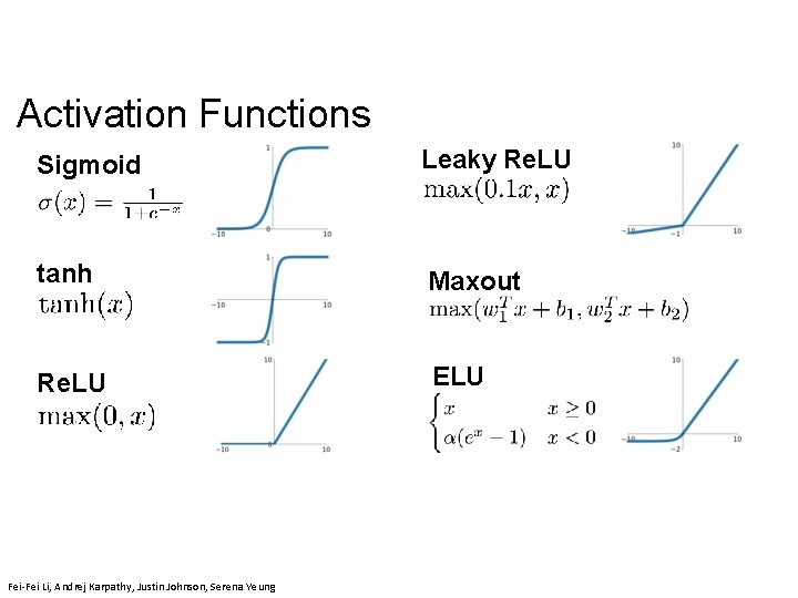
Activation Functions Sigmoid Leaky Re. LU tanh Maxout Re. LU ELU Fei-Fei Li & Justin Johnson & Serena Yeung Fei-Fei Li, Andrej Karpathy, Justin Johnson, Serena Yeung Lecture 7 - April 22, 2019
![Activation Functions Squashes numbers to range 0 1 Historically popular since they Activation Functions - Squashes numbers to range [0, 1] - Historically popular since they](https://slidetodoc.com/presentation_image_h2/9895368f71e9327388947d823a2357bc/image-11.jpg)
Activation Functions - Squashes numbers to range [0, 1] - Historically popular since they have nice interpretation as a saturating “firing rate” of a neuron Sigmoid Fei-Fei Li & Justin Johnson & Serena Yeung Fei-Fei Li, Andrej Karpathy, Justin Johnson, Serena Yeung
![Activation Functions Squashes numbers to range 0 1 Historically popular since they Activation Functions - Squashes numbers to range [0, 1] - Historically popular since they](https://slidetodoc.com/presentation_image_h2/9895368f71e9327388947d823a2357bc/image-12.jpg)
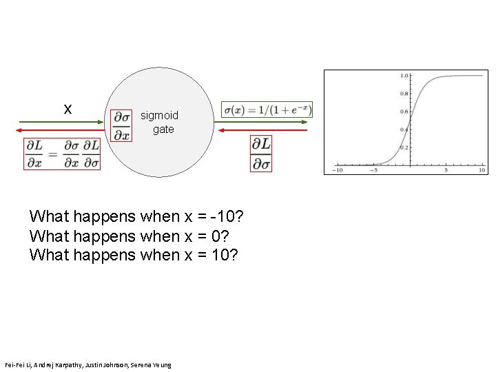
Activation Functions - Squashes numbers to range [0, 1] - Historically popular since they have nice interpretation as a saturating “firing rate” of a neuron • 3 problems: Sigmoid 1. Saturated neurons “kill” the gradients Fei-Fei Li & Justin Johnson & Serena Yeung Fei-Fei Li, Andrej Karpathy, Justin Johnson, Serena Yeung 12 Lecture 7 - April 22, 2019

x sigmoid gate What happens when x = -10? What happens when x = 10? Fei-Fei Li & Justin Johnson & Serena Yeung Fei-Fei Li, Andrej Karpathy, Justin Johnson, Serena Yeung 13 Lecture 7 - April 22, 2019
![Activation Functions Squashes numbers to range 0 1 Historically popular since they Activation Functions - Squashes numbers to range [0, 1] - Historically popular since they](https://slidetodoc.com/presentation_image_h2/9895368f71e9327388947d823a2357bc/image-14.jpg)
Activation Functions - Squashes numbers to range [0, 1] - Historically popular since they have nice interpretation as a saturating “firing rate” of a neuron • 3 problems: 1. Saturated neurons “kill” the gradients Sigmoid 2. Sigmoid outputs are not Fei-Fei Li & Justin Johnson & Serena Yeung zero-centered 14 April 22, 2019 Fei-Fei Li & Justin Johnson & Serena Yeung Fei-Fei Li, Andrej Karpathy, Justin Johnson, Serena Yeung Lecture 7 - April 22, 2019
![Activation Functions Squashes numbers to range 0 1 Historically popular since they Activation Functions - Squashes numbers to range [0, 1] - Historically popular since they](https://slidetodoc.com/presentation_image_h2/9895368f71e9327388947d823a2357bc/image-15.jpg)
Activation Functions - Squashes numbers to range [0, 1] - Historically popular since they have nice interpretation as a saturating “firing rate” of a neuron • 3 problems: 1. Saturated neurons “kill” the gradients Sigmoid 2. Sigmoid outputs are not Fei-Fei Li & Justin Johnson & Serena Yeung April 22, 2019 zero-centered 3. exp() is a bit compute expensive Fei-Fei Li & Justin Johnson & Serena Yeung Fei-Fei Li, Andrej Karpathy, Justin Johnson, Serena Yeung Lecture 7 - April 22, 2019
![Activation Functions Squashes numbers to range 1 1 zero centered nice Activation Functions - Squashes numbers to range [-1, 1] - zero centered (nice) -](https://slidetodoc.com/presentation_image_h2/9895368f71e9327388947d823a2357bc/image-16.jpg)
Activation Functions - Squashes numbers to range [-1, 1] - zero centered (nice) - still kills gradients when saturated : ( tanh(x) April 22, 2019 Fei-Fei Li & Justin Johnson & Serena Yeung [Le. Cun et al. , 1991] Fei-Fei Li & Justin Johnson & Serena Yeung Fei-Fei Li, Andrej Karpathy, Justin Johnson, Serena Yeung Lecture 7 - April 22, 2019

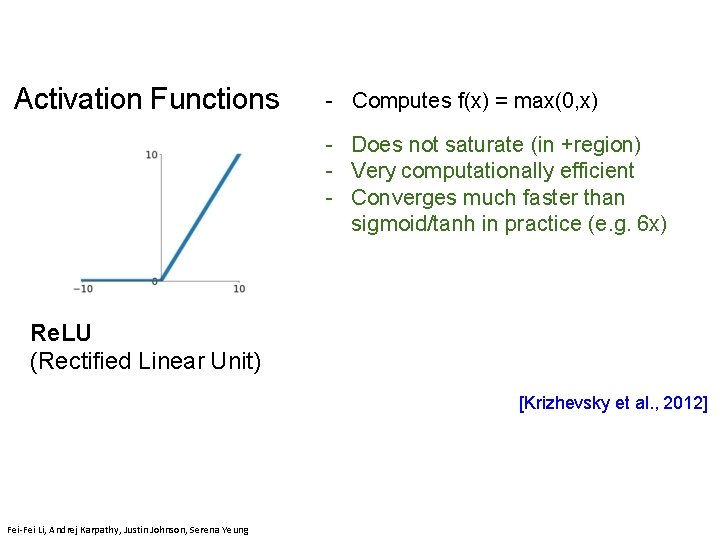
Activation Functions - Computes f(x) = max(0, x) - Does not saturate (in +region) - Very computationally efficient - Converges much faster than sigmoid/tanh in practice (e. g. 6 x) Re. LU (Rectified Linear Unit) April 22, 2019 Fei-Fei Li & Justin Johnson & Serena Yeung [Krizhevsky et al. , 2012] Fei-Fei Li & Justin Johnson & Serena Yeung Fei-Fei Li, Andrej Karpathy, Justin Johnson, Serena Yeung Lecture 7 - April 22, 2019

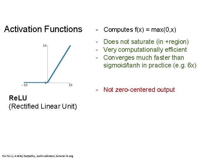
Activation Functions - Computes f(x) = max(0, x) - Does not saturate (in +region) - Very computationally efficient - Converges much faster than sigmoid/tanh in practice (e. g. 6 x) - Not zero-centered output Re. LU (Rectified Linear Unit) Fei-Fei Li & Justin Johnson & Serena Yeung Fei-Fei Li, Andrej Karpathy, Justin Johnson, Serena Yeung Lecture 7 - April 22, 2019

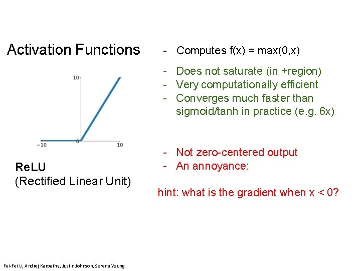
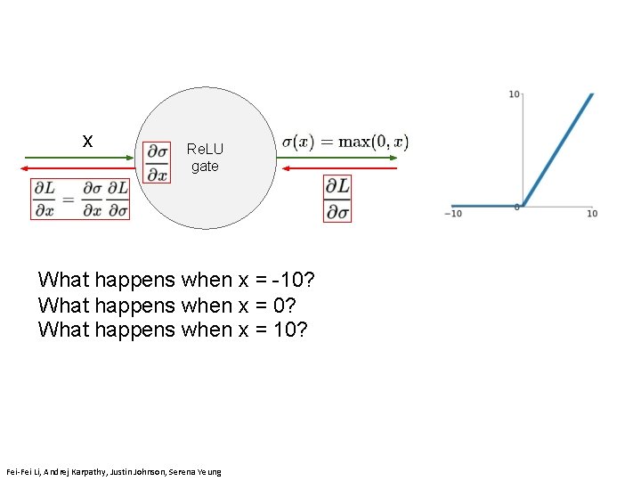
Activation Functions - Computes f(x) = max(0, x) - Does not saturate (in +region) - Very computationally efficient - Converges much faster than sigmoid/tanh in practice (e. g. 6 x) Re. LU (Rectified Linear Unit) - Not zero-centered output - An annoyance: hint: what is the gradient when x < 0? Fei-Fei Li & Justin Johnson & Serena Yeung Fei-Fei Li, Andrej Karpathy, Justin Johnson, Serena Yeung Lecture 7 - April 22, 2019

x Re. LU gate What happens when x = -10? What happens when x = 10? Fei-Fei Li & Justin Johnson & Serena Yeung Fei-Fei Li, Andrej Karpathy, Justin Johnson, Serena Yeung 20 Lecture 7 - April 22, 2019
![Mass et al 2013 He et al 2015 Activation Functions Does [Mass et al. , 2013] [He et al. , 2015] Activation Functions - Does](https://slidetodoc.com/presentation_image_h2/9895368f71e9327388947d823a2357bc/image-21.jpg)
[Mass et al. , 2013] [He et al. , 2015] Activation Functions - Does not saturate - Computationally efficient - Converges much faster than sigmoid/tanh in practice! (e. g. 6 x) - will not “die”. Leaky Re. LU 21 Fei-Fei Li & Justin Johnson & Serena Yeung Fei-Fei Li, Andrej Karpathy, Justin Johnson, Serena Yeung Lecture 7 - April 22, 2019
![Mass et al 2013 He et al 2015 Activation Functions Does [Mass et al. , 2013] [He et al. , 2015] Activation Functions - Does](https://slidetodoc.com/presentation_image_h2/9895368f71e9327388947d823a2357bc/image-22.jpg)
[Mass et al. , 2013] [He et al. , 2015] Activation Functions - Does not saturate - Computationally efficient - Converges much faster than sigmoid/tanh in practice! (e. g. 6 x) - will not “die”. Leaky Re. LU Parametric Rectifier (PRe. LU) Fei-Fei Li & Justin Johnson & Serena Yeung backprop into alpha (parameter) Fei-Fei Li & Justin Johnson & Serena Yeung Fei-Fei Li, Andrej Karpathy, Justin Johnson, Serena Yeung Lecture 7 - April 22, 2019
![Clevert et al 2015 Activation Functions Exponential Linear Units ELU All benefits [Clevert et al. , 2015] Activation Functions Exponential Linear Units (ELU) - All benefits](https://slidetodoc.com/presentation_image_h2/9895368f71e9327388947d823a2357bc/image-23.jpg)
[Clevert et al. , 2015] Activation Functions Exponential Linear Units (ELU) - All benefits of Re. LU - Closer to zero mean outputs - Negative saturation regime compared with Leaky Re. LU adds some robustness to noise - Computation requires exp() Fei-Fei Li & Justin Johnson & Serena Yeung Fei-Fei Li, Andrej Karpathy, Justin Johnson, Serena Yeung Lecture 7 - April 22, 2019
![Goodfellow et al 2013 Maxout Neuron Does not have the basic form [Goodfellow et al. , 2013] Maxout “Neuron” - Does not have the basic form](https://slidetodoc.com/presentation_image_h2/9895368f71e9327388947d823a2357bc/image-24.jpg)
[Goodfellow et al. , 2013] Maxout “Neuron” - Does not have the basic form of dot product -> nonlinearity - Generalizes Re. LU and Leaky Re. LU - Linear Regime! Does not saturate! Does not die! Problem: doubles the number of parameters/neuron : ( Fei-Fei Li & Justin Johnson & Serena Yeung Fei-Fei Li, Andrej Karpathy, Justin Johnson, Serena Yeung 24 Lecture 7 - April 22, 2019

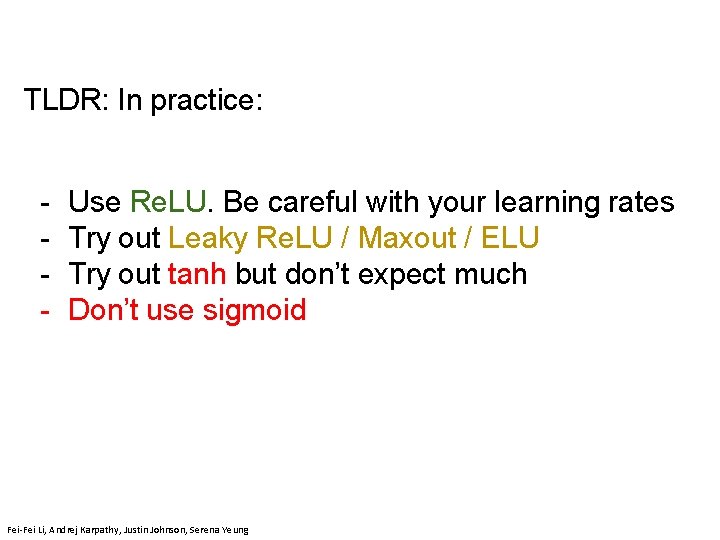
TLDR: In practice: - Use Re. LU. Be careful with your learning rates Try out Leaky Re. LU / Maxout / ELU Try out tanh but don’t expect much Don’t use sigmoid Fei-Fei Li & Justin Johnson & Serena Yeung Fei-Fei Li, Andrej Karpathy, Justin Johnson, Serena Yeung 25 Lecture 7 - April 22, 2019
![Batch Normalization Ioffe and Szegedy 2015 you want zeromean unitvariance activations just make them Batch Normalization [Ioffe and Szegedy, 2015] “you want zero-mean unit-variance activations? just make them](https://slidetodoc.com/presentation_image_h2/9895368f71e9327388947d823a2357bc/image-26.jpg)
Batch Normalization [Ioffe and Szegedy, 2015] “you want zero-mean unit-variance activations? just make them so. ” consider a batch of activations at some layer. To make each dimension zero-mean unit-variance, apply: April 19, 62018 Lecture - 26 Fei-Fei Li & Justin Johnson & Serena Yeung Fei-Fei Li, Andrej Karpathy, Justin Johnson, Serena Yeung Lecture 6 - April 19, 2018
![Batch Normalization Ioffe and Szegedy 2015 you want zeromean unitvariance activations just make them Batch Normalization [Ioffe and Szegedy, 2015] “you want zero-mean unit-variance activations? just make them](https://slidetodoc.com/presentation_image_h2/9895368f71e9327388947d823a2357bc/image-27.jpg)
Batch Normalization [Ioffe and Szegedy, 2015] “you want zero-mean unit-variance activations? just make them so. ” 1. compute the empirical mean and variance independently for each dimension. N 2. Normalize April 19, 2018 D Fei-Fei Li & Justin Johnson & Serena Yeung Fei-Fei Li, Andrej Karpathy, Justin Johnson, Serena Yeung Lecture 6 - April 19, 2018
![Batch Normalization Ioffe and Szegedy 2015 Normalize Note the network can learn And then Batch Normalization [Ioffe and Szegedy, 2015] Normalize: Note, the network can learn: And then](https://slidetodoc.com/presentation_image_h2/9895368f71e9327388947d823a2357bc/image-28.jpg)
Batch Normalization [Ioffe and Szegedy, 2015] Normalize: Note, the network can learn: And then allow the network to squash the range if it wants to: to recover the identity mapping. Fei-Fei Li & Justin Johnson & Serena Yeung Fei-Fei Li, Andrej Karpathy, Justin Johnson, Serena Yeung Lecture 6 - April 19, 2018
![Batch Normalization Ioffe and Szegedy 2015 Improves gradient flow through the network Batch Normalization [Ioffe and Szegedy, 2015] - Improves gradient flow through the network -](https://slidetodoc.com/presentation_image_h2/9895368f71e9327388947d823a2357bc/image-29.jpg)
Batch Normalization [Ioffe and Szegedy, 2015] - Improves gradient flow through the network - Allows higher learning rates - Reduces the strong dependence on initialization - Acts as a form of regularization Fei-Fei Li & Justin Johnson & Serena Yeung Fei-Fei Li, Andrej Karpathy, Justin Johnson, Serena Yeung Lecture 6 - 29 April 19, 2018 Lecture 6 - April 19, 2018
![Batch Normalization Ioffe and Szegedy 2015 Note at test time Batch Norm layer functions Batch Normalization [Ioffe and Szegedy, 2015] Note: at test time Batch. Norm layer functions](https://slidetodoc.com/presentation_image_h2/9895368f71e9327388947d823a2357bc/image-30.jpg)
Batch Normalization [Ioffe and Szegedy, 2015] Note: at test time Batch. Norm layer functions differently: The mean/std are not computed based on the batch. Instead, a single fixed empirical mean of activations during training is used. (e. g. can be estimated during training with running averages) Fei-Fei Li & Justin Johnson & Serena Yeung Lecture 6 - 30 April 19, 2018 Fei-Fei Li & Justin Johnson & Serena Yeung Lecture 6 - April 19, 2018 Fei-Fei Li, Andrej Karpathy, Justin Johnson, Serena Yeung

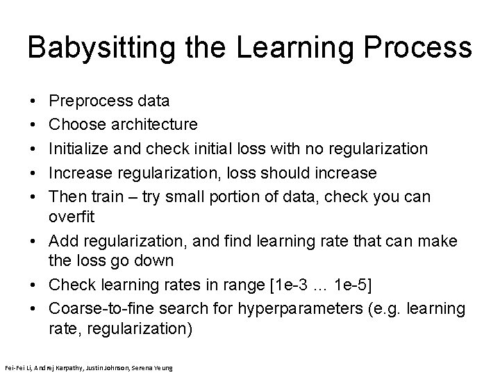
Babysitting the Learning Process • • • Preprocess data Choose architecture Initialize and check initial loss with no regularization Increase regularization, loss should increase Then train – try small portion of data, check you can overfit • Add regularization, and find learning rate that can make the loss go down • Check learning rates in range [1 e-3 … 1 e-5] • Coarse-to-fine search for hyperparameters (e. g. learning rate, regularization) Fei-Fei Li, Andrej Karpathy, Justin Johnson, Serena Yeung

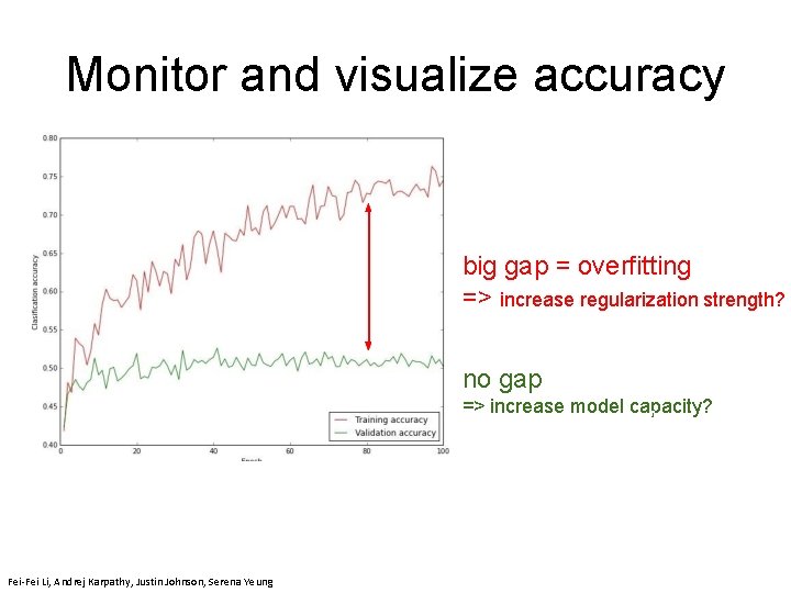
Monitor and visualize accuracy big gap = overfitting => increase regularization strength? no gap => increase model capacity? April 19, 2018 Fei-Fei Li & Justin Johnson & Serena Yeung Fei-Fei Li, Andrej Karpathy, Justin Johnson, Serena Yeung Lecture 6 - April 19, 2018

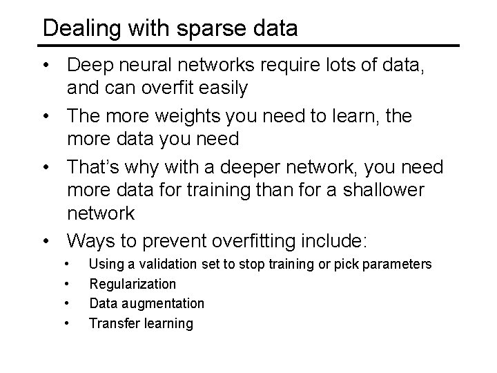
Dealing with sparse data • Deep neural networks require lots of data, and can overfit easily • The more weights you need to learn, the more data you need • That’s why with a deeper network, you need more data for training than for a shallower network • Ways to prevent overfitting include: • • Using a validation set to stop training or pick parameters Regularization Data augmentation Transfer learning

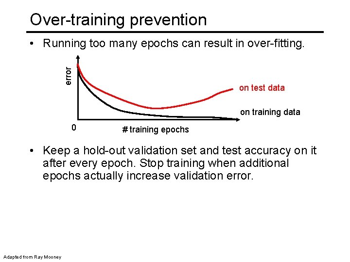
Over-training prevention error • Running too many epochs can result in over-fitting. on test data on training data 0 # training epochs • Keep a hold-out validation set and test accuracy on it after every epoch. Stop training when additional epochs actually increase validation error. Adapted from Ray Mooney

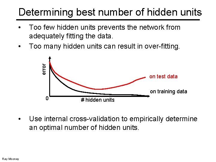
Determining best number of hidden units • error • Too few hidden units prevents the network from adequately fitting the data. Too many hidden units can result in over-fitting. on test data on training data 0 • Ray Mooney # hidden units Use internal cross-validation to empirically determine an optimal number of hidden units.

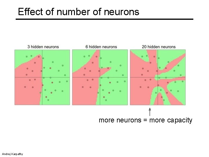
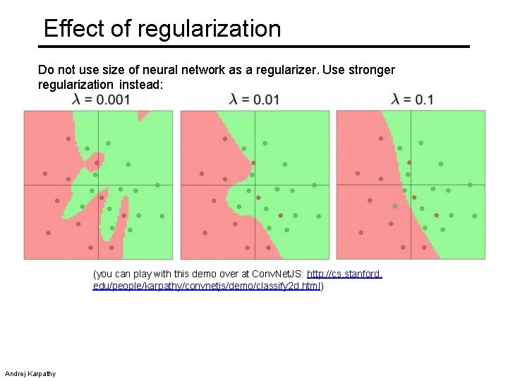
Effect of number of neurons more neurons = more capacity Andrej Karpathy

Effect of regularization Do not use size of neural network as a regularizer. Use stronger regularization instead: (you can play with this demo over at Conv. Net. JS: http: //cs. stanford. edu/people/karpathy/convnetjs/demo/classify 2 d. html) Andrej Karpathy

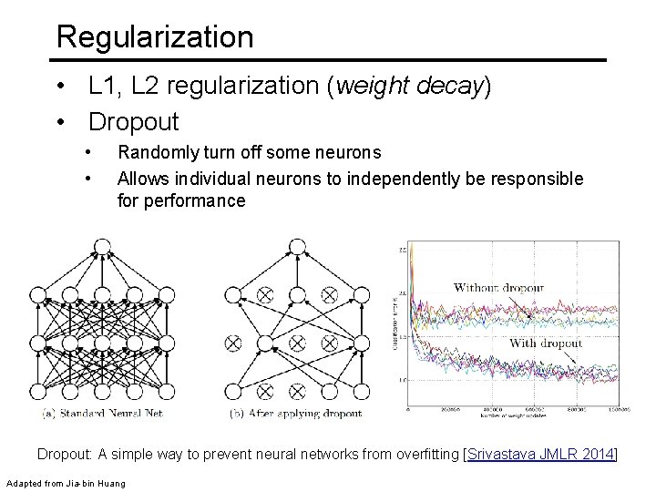
Regularization • L 1, L 2 regularization (weight decay) • Dropout • • Randomly turn off some neurons Allows individual neurons to independently be responsible for performance Dropout: A simple way to prevent neural networks from overfitting [Srivastava JMLR 2014] Adapted from Jia-bin Huang

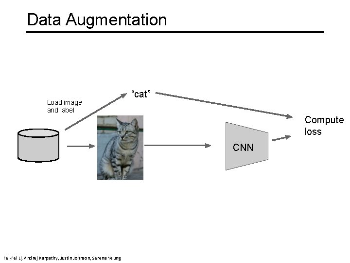
Data Augmentation “cat” Load image and label Compute loss CNN Fei-Fei Li & Justin Johnson & Serena Yeung April 24, 2018 Fei-Fei Li, Andrej Karpathy, Justin Johnson, Serena Yeung Lecture 7 - April 24, 2018 Lecture 7 - 39

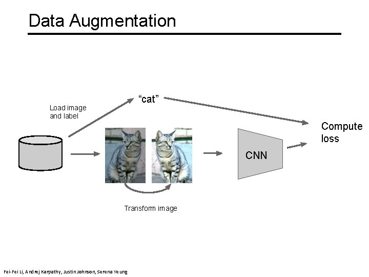
Data Augmentation “cat” Load image and label Compute loss CNN Transform image Fei-Fei Li & Justin Johnson & Serena Yeung April 24, 2018 Fei-Fei Li, Andrej Karpathy, Justin Johnson, Serena Yeung Lecture 7 - April 24, 2018 Lecture 7 - 40

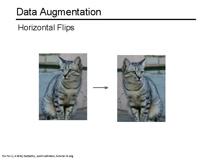
Data Augmentation Horizontal Flips Fei-Fei Li & Justin Johnson & Serena Yeung Fei-Fei Li & Justin April 24, 2018 Johnson & Serena Fei-Fei Li, Andrej Karpathy, Justin Johnson, Serena Yeung Lecture 7 - April 24, 2018 Lecture 7 - 41

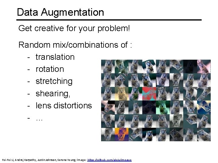
Data Augmentation Get creative for your problem! Random mix/combinations of : - translation - rotation - stretching - shearing, - lens distortions - … Fei-Fei Li & Justin Johnson & Serena Yeung Lecture 7 - April 24, 2018 Fei-Fei Li, Andrej Karpathy, Justin Johnson, Serena Yeung; Image: https: //github. com/aleju/imgaug April 24, 2018 Lecture 7 - 42

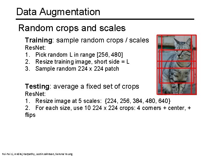
Data Augmentation Random crops and scales Training: sample random crops / scales Res. Net: 1. Pick random L in range [256, 480] 2. Resize training image, short side = L 3. Sample random 224 x 224 patch Testing: average a fixed set of crops Res. Net: 1. Resize image at 5 scales: {224, 256, 384, 480, 640} 2. For each size, use 10 224 x 224 crops: 4 corners + center, + flips Fei-Fei Li & Justin Johnson & Serena Yeung April 24, 2018 Fei-Fei Li, Andrej Karpathy, Justin Johnson, Serena Yeung Lecture 7 - April 24, 2018 Lecture 7 - 43

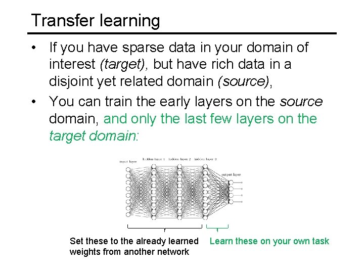
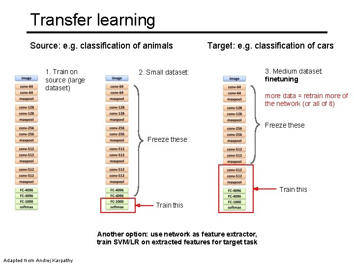
Transfer learning • If you have sparse data in your domain of interest (target), but have rich data in a disjoint yet related domain (source), • You can train the early layers on the source domain, and only the last few layers on the target domain: Set these to the already learned weights from another network Learn these on your own task

Transfer learning Source: e. g. classification of animals 1. Train on source (large dataset) Target: e. g. classification of cars 2. Small dataset: 3. Medium dataset: finetuning more data = retrain more of the network (or all of it) Freeze these Train this Lecture 11 Another option: use network as feature extractor, train SVM/LR on extracted features for target task Adapted from Andrej Karpathy 29

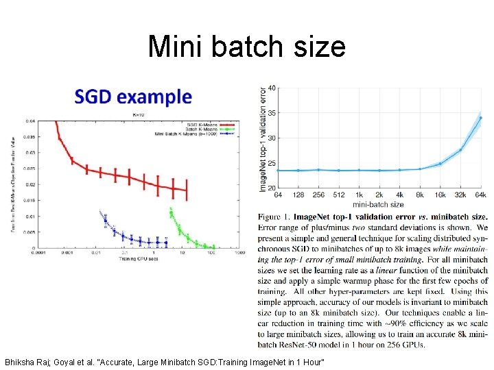
Mini-batch gradient descent • In classic gradient descent, we compute the gradient from the loss for all training examples • Could also only use some of the data for each gradient update • We cycle through all the training examples multiple times • Each time we’ve cycled through all of them once is called an ‘epoch’ • Allows faster training (e. g. on GPUs), parallelization

Training: Best practices • Center (subtract mean from) your data • To initialize weights, use “Xavier initialization” • Use RELU or leaky RELU or ELU, don’t use sigmoid • Use mini-batch • Use data augmentation • Use regularization • Use batch normalization • Use cross-validation for your parameters • Learning rate: too high? Too low?

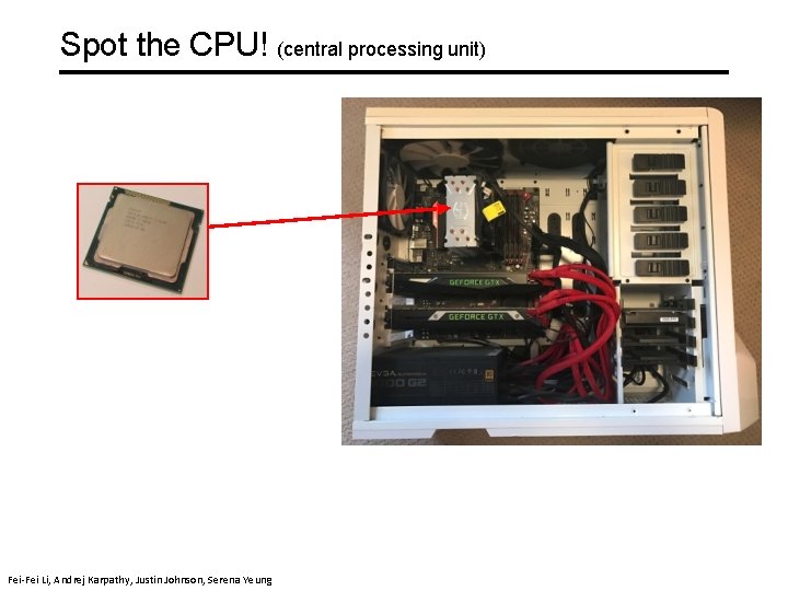
Spot the CPU! (central processing unit) Fei-Fei Li & Justin Johnson & Serena Yeung Fei-Fei Li, Andrej Karpathy, Justin Johnson, Serena Yeung

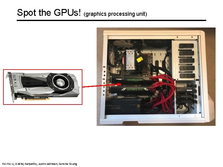
Spot the GPUs! (graphics processing unit) Fei-Fei Li & Justin Johnson & Serena Yeung Lecture 8 - April 26, 2018 Fei-Fei Li, Andrej Karpathy, Justin Johnson, Serena Yeung

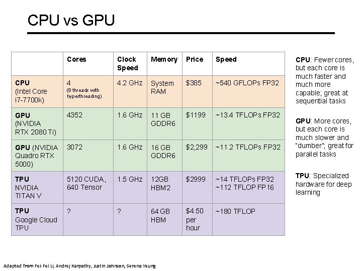
CPU vs GPU Cores Clock Speed Memory Price Speed CPU (Intel Core i 7 -7700 k) 4 4. 2 GHz System RAM $385 ~540 GFLOPs FP 32 GPU (NVIDIA RTX 2080 Ti) 4352 1. 6 GHz 11 GB GDDR 6 $1199 ~13. 4 TFLOPs FP 32 GPU (NVIDIA Quadro RTX 5000) 3072 1. 6 GHz 16 GB GDDR 6 $2, 299 ~11. 2 TFLOPs FP 32 TPU NVIDIA TITAN V 5120 CUDA, 640 Tensor 1. 5 GHz 12 GB HBM 2 $2999 ~14 TFLOPs FP 32 ~112 TFLOP FP 16 ? 64 GB HBM $4. 50 per hour ~180 TFLOP (8 threads with hyperthreading) TPU ? Google Cloud Fei-Fei TPU Li & Justin Johnson & Serena Yeung Adapted from Fei-Fei Li, Andrej Karpathy, Justin Johnson, Serena Yeung CPU: Fewer cores, but each core is much faster and much more capable; great at sequential tasks GPU: More cores, but each core is much slower and “dumber”; great for parallel tasks TPU: Specialized hardware for deep learning

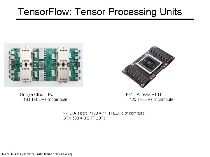
Tensor. Flow: Tensor Processing Units Google Cloud TPU = 180 TFLOPs of compute! NVIDIA Tesla V 100 = 125 TFLOPs of compute April 18, 2019 Fei-Fei Li & Justin Johnson. NVIDIA & Serena Tesla Yeung P 100 = 11 TFLOPs of compute GTX 580 = 0. 2 TFLOPs Lecture 6 - Fei-Fei Li, Andrej Karpathy, Justin Johnson, Serena Yeung 51

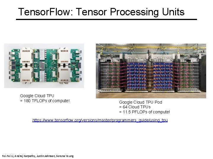
Tensor. Flow: Tensor Processing Units Google Cloud TPU = 180 TFLOPs of compute! Fei-Fei Li & Justin Johnson & Serena Yeung Google Cloud TPU Pod = 64 Cloud TPUs = 11. 5 PFLOPs of compute! https: //www. tensorflow. org/versions/master/programmers_guide/using_tpu Lecture 6 - Fei-Fei Li, Andrej Karpathy, Justin Johnson, Serena Yeung 52 April 18, 2019

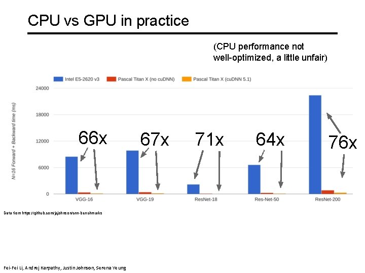
CPU vs GPU in practice (CPU performance not well-optimized, a little unfair) 66 x 67 x 71 x 64 x 76 x Data from https: //github. com/jcjohnson/cnn-benchmarks Fei-Fei Li & Justin Johnson & Serena Yeung Fei-Fei Li, Andrej Karpathy, Justin Johnson, Serena Yeung Lecture 8 - April 26, 2018

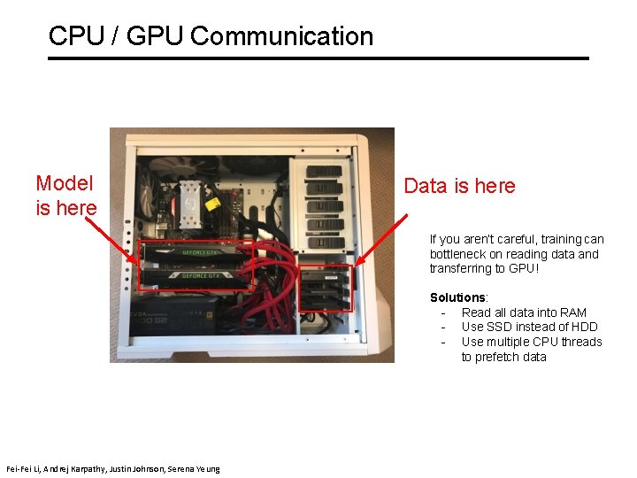
CPU / GPU Communication Model is here Data is here If you aren’t careful, training can bottleneck on reading data and transferring to GPU! Solutions: - Read all data into RAM - Use SSD instead of HDD Lecture 26, 2018 8 - Use multiple. April CPU threads to prefetch data Fei-Fei Li & Justin Johnson & Serena Yeung Fei-Fei Li, Andrej Karpathy, Justin Johnson, Serena Yeung Lecture 8 - April 26, 2018

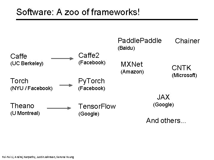
Software: A zoo of frameworks! Paddle Chainer (Baidu) Caffe (UC Berkeley) Caffe 2 (Facebook) MXNet CNTK (Amazon) Torch Py. Torch (NYU / Facebook) (Microsoft) JAX Theano (U Montreal) Tensor. Flow (Google) Fei-Fei Li & Justin Johnson & Serena Yeung Fei-Fei Li, Andrej Karpathy, Justin Johnson, Serena Yeung (Google) And others. . . Lecture 8 - April 26, 2018

Convergence of training

Successful training • We want training to converge (stop) at a reasonable place • Stopping is not guaranteed – e. g. imagine taking larger and larger steps… • Stopping in a good place is not guaranteed

Loss surfaces • Usually Loss(W) is not convex, so there are many local minima • However, in deep networks, these minima are reasonably similar – not true in small networks • What are desirable properties of the loss surface?

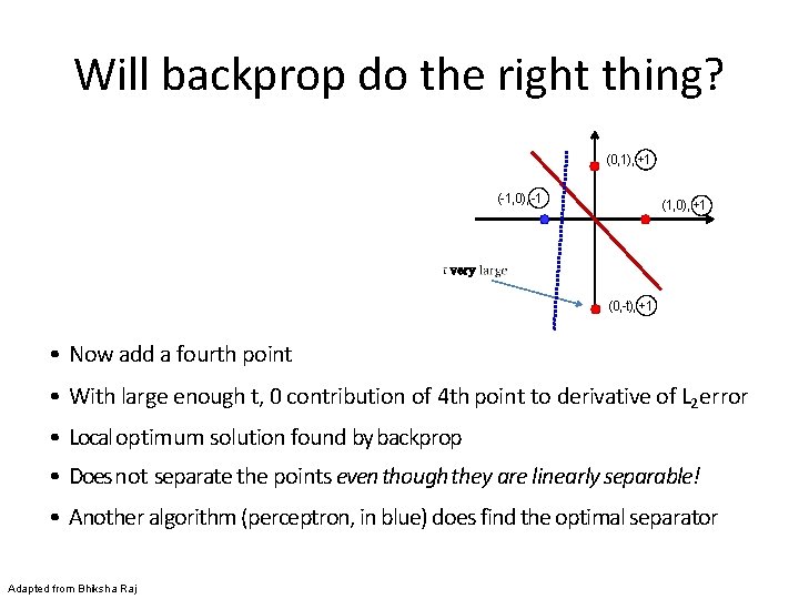
Will backprop do the right thing? • In classification problems, the classification error is a non-differentiable function of weights • The divergence function minimized is only a proxy for classification error • Minimizing divergence may not minimize classification error Bhiksha Raj

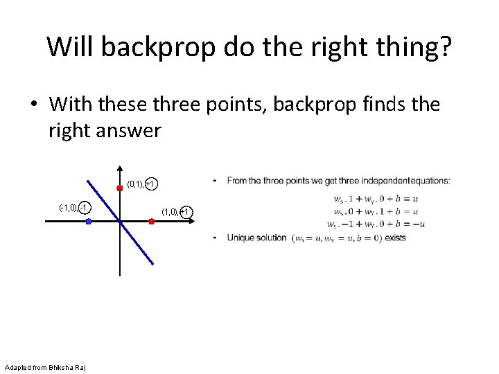
Will backprop do the right thing? • With these three points, backprop finds the right answer (0, 1), +1 (-1, 0), -1 Adapted from Bhiksha Raj (1, 0), +1

Will backprop do the right thing? (0, 1), +1 (-1, 0), -1 (1, 0), +1 (0, -t), +1 • Now add a fourth point • With large enough t, 0 contribution of 4 th point to derivative of L 2 error • Local optimum solution found by backprop • Does not separate the points even though they are linearly separable! • Another algorithm (perceptron, in blue) does find the optimal separator Adapted from Bhiksha Raj

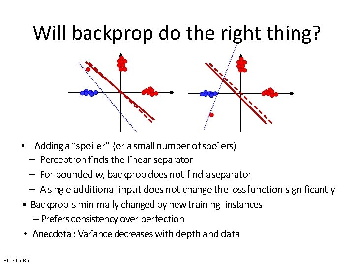
Will backprop do the right thing? • Adding a “spoiler” (or a small number of spoilers) – Perceptron finds the linear separator – For bounded w, backprop does not find aseparator – A single additional input does not change the loss function significantly • Backprop is minimally changed by new training instances – Prefers consistency over perfection • Anecdotal: Variance decreases with depth and data Bhiksha Raj

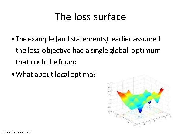
The loss surface • The example (and statements) earlier assumed the loss objective had a single global optimum that could be found • What about local optima? Adapted from Bhiksha Raj

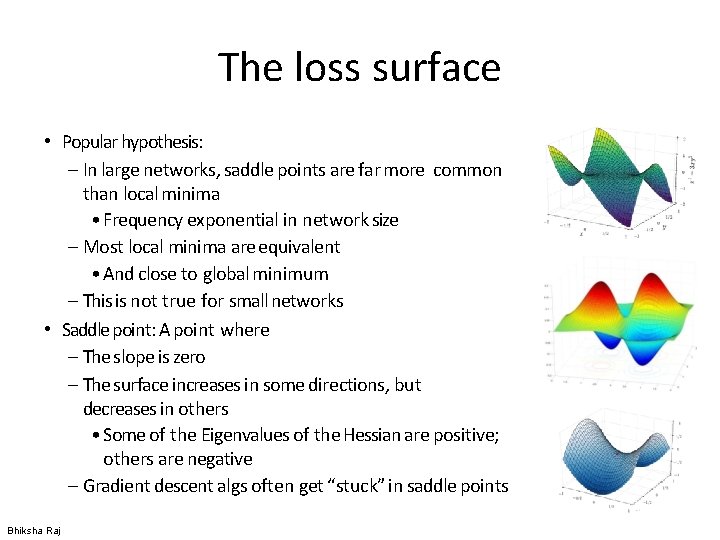
The loss surface • Popular hypothesis: – In large networks, saddle points are far more common than local minima • Frequency exponential in network size – Most local minima are equivalent • And close to global minimum – This is not true for small networks • Saddle point: A point where – The slope is zero – The surface increases in some directions, but decreases in others • Some of the Eigenvalues of the Hessian are positive; others are negative – Gradient descent algs often get “stuck” in saddle points Bhiksha Raj

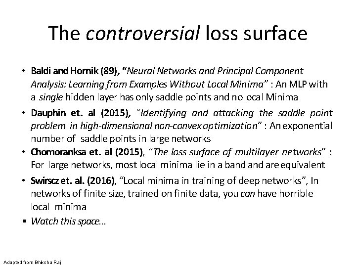
The controversial loss surface • Baldi and Hornik (89), “Neural Networks and Principal Component Analysis: Learning from Examples Without Local Minima” : An MLP with a single hidden layer has only saddle points and no local Minima • Dauphin et. al (2015), “Identifying and attacking the saddle point problem in high-dimensional non-convex optimization” : An exponential number of saddle points in large networks • Chomoranksa et. al (2015), “The loss surface of multilayer networks” : For large networks, most local minima lie in a band are equivalent • Swirscz et. al. (2016), “Local minima in training of deep networks”, In networks of finite size, trained on finite data, you can have horrible local minima • Watch this space… Adapted from Bhiksha Raj

Conditions for convergence • In the discussion so far we have assumed the training arrives at a local minimum • Does it always converge? • How long does it take? • Hard to analyze for a neural network, but we can look at the problem through the lens of convex optimization Adapted from Bhiksha Raj

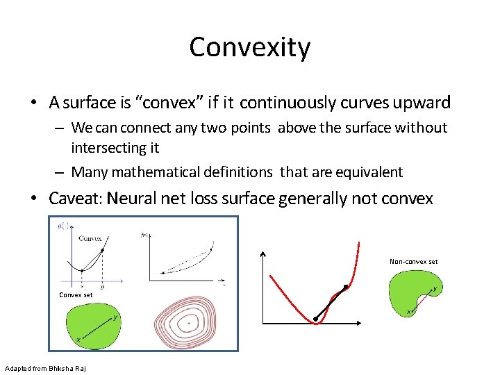
Convexity • A surface is “convex” if it continuously curves upward – We can connect any two points above the surface without intersecting it – Many mathematical definitions that are equivalent • Caveat: Neural net loss surface generally not convex Non-convex set Convex set Adapted from Bhiksha Raj

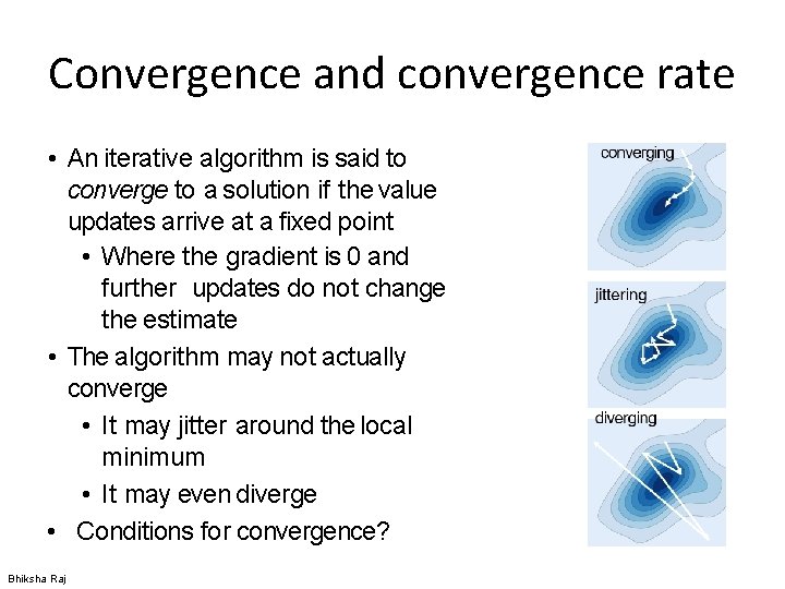
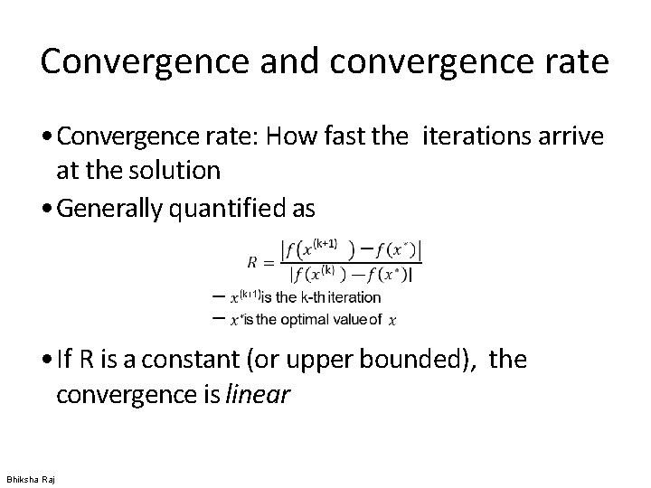
Convergence and convergence rate • An iterative algorithm is said to converge to a solution if the value updates arrive at a fixed point • Where the gradient is 0 and further updates do not change the estimate • The algorithm may not actually converge • It may jitter around the local minimum • It may even diverge • Conditions for convergence? Bhiksha Raj

Convergence and convergence rate • Convergence rate: How fast the iterations arrive at the solution • Generally quantified as • If R is a constant (or upper bounded), the convergence is linear Bhiksha Raj

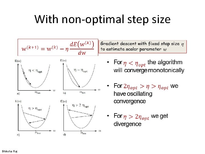
With non-optimal step size Bhiksha Raj

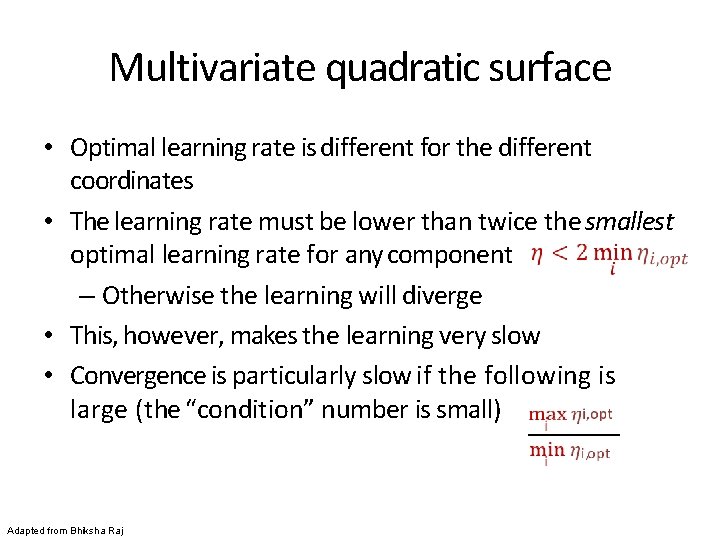
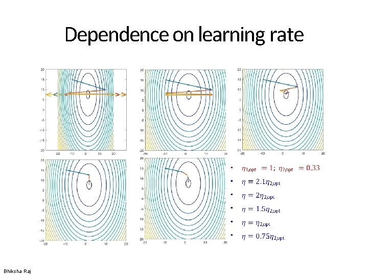
Multivariate quadratic surface • Optimal learning rate is different for the different coordinates • The learning rate must be lower than twice the smallest optimal learning rate for any component – Otherwise the learning will diverge • This, however, makes the learning very slow • Convergence is particularly slow if the following is large (the “condition” number is small) Adapted from Bhiksha Raj

Dependence on learning rate Bhiksha Raj

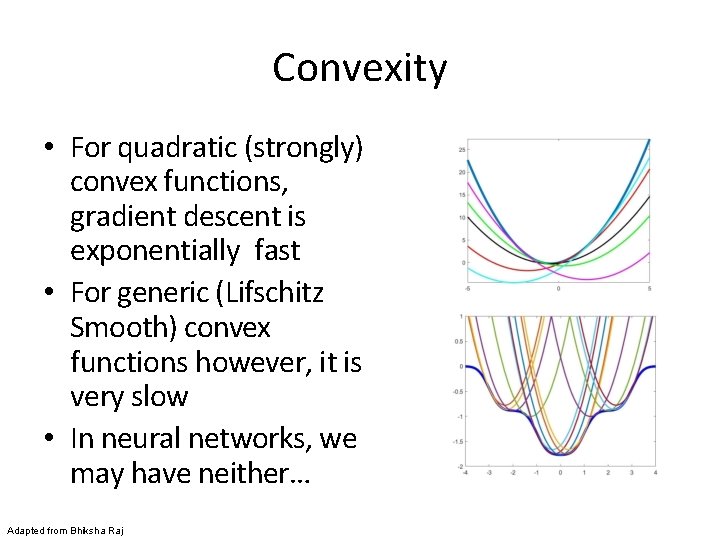
Convexity • For quadratic (strongly) convex functions, gradient descent is exponentially fast • For generic (Lifschitz Smooth) convex functions however, it is very slow • In neural networks, we may have neither… Adapted from Bhiksha Raj

Optimization strategies

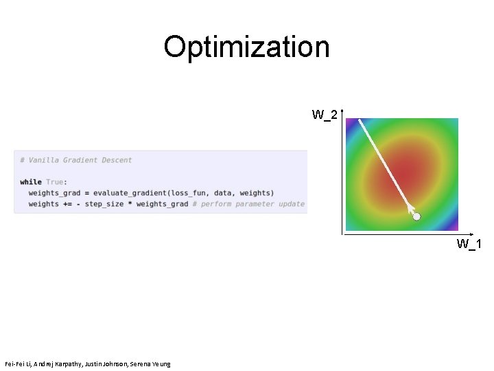
Getting to the minimum • Gradient descent is just one strategy, but has several problems • What other “steps” can we take? • How far in the direction of decreasing gradient do we go? With what speed/acceleration? • What about overshooting minima?

Optimization W_2 W_1 Fei-Fei Li & Justin Johnson & Serena Yeung Lecture 7 - 76 April 24, 2018 Fei-Fei Li & Justin Johnson & Serena Yeung Lecture 7 - April 24, 2018 Fei-Fei Li, Andrej Karpathy, Justin Johnson, Serena Yeung

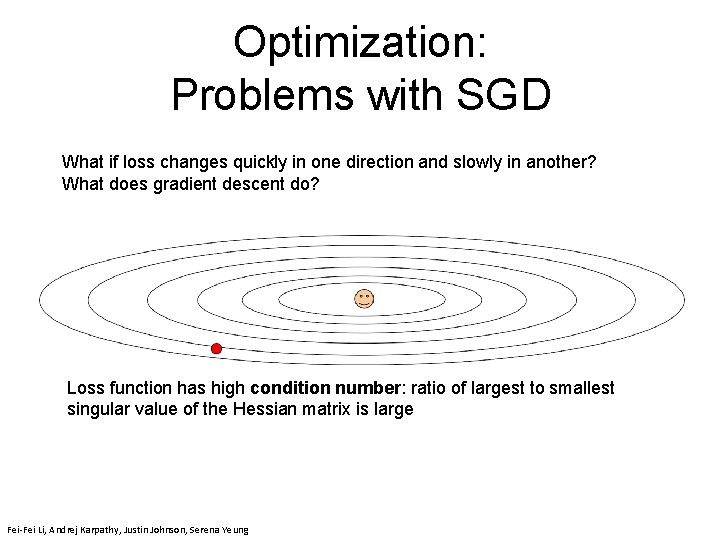
Optimization: Problems with SGD What if loss changes quickly in one direction and slowly in another? What does gradient descent do? Loss function has high condition number: ratio of largest to smallest singular value of the Hessian matrix is large Fei-Fei Li & Justin Johnson & Serena Yeung Fei-Fei Li, Andrej Karpathy, Justin Johnson, Serena Yeung Lecture 7 - April 24, 2018

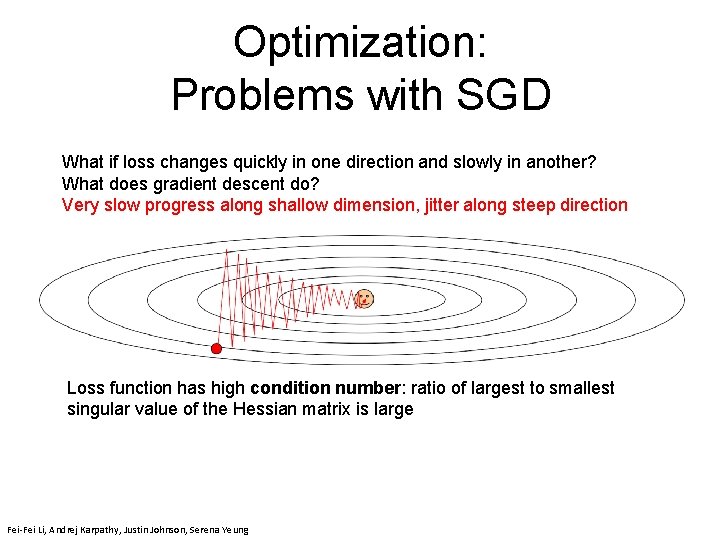
Optimization: Problems with SGD What if loss changes quickly in one direction and slowly in another? What does gradient descent do? Very slow progress along shallow dimension, jitter along steep direction Loss function has high condition number: ratio of largest to smallest singular value of the Hessian matrix is large Fei-Fei Li & Justin Johnson & Serena Yeung Fei-Fei Li, Andrej Karpathy, Justin Johnson, Serena Yeung Lecture 7 - April 24, 2018

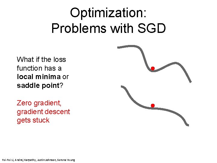
Optimization: Problems with SGD What if the loss function has a local minima or saddle point? Zero gradient, gradient descent gets stuck Fei-Fei Li & Justin Johnson & Serena Yeung Fei-Fei Li, Andrej Karpathy, Justin Johnson, Serena Yeung Lecture 7 - 79 Lecture 7 - April 24, 2018

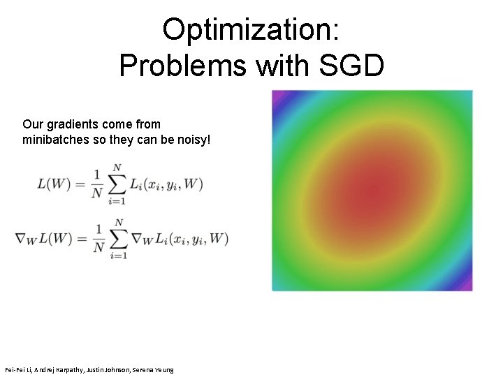
Optimization: Problems with SGD Our gradients come from minibatches so they can be noisy! Fei-Fei Li & Justin Johnson & Serena Yeung Fei-Fei Li, Andrej Karpathy, Justin Johnson, Serena Yeung Lecture 7 - April 24, 2018

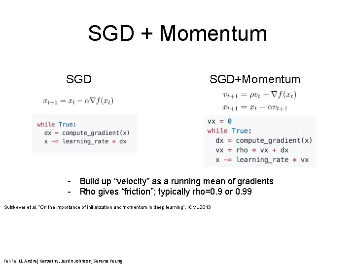
SGD + Momentum SGD+Momentum - Build up “velocity” as a running mean of gradients - Rho gives “friction”; typically rho=0. 9 or 0. 99 April 24, 72018 Lecture - 81 Sutskever et al, “On the importance of initialization and momentum in deep learning”, ICML 2013 Fei-Fei Li & Justin Johnson & Serena Yeung Fei-Fei Li, Andrej Karpathy, Justin Johnson, Serena Yeung Lecture 7 - April 24, 2018

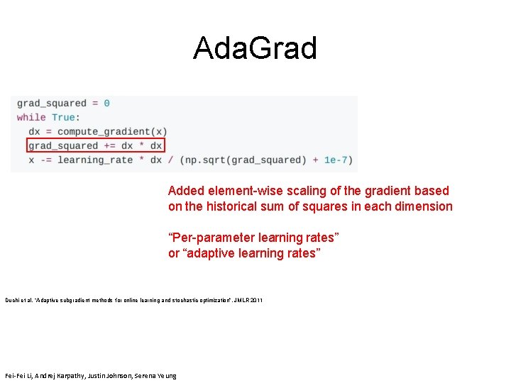
Ada. Grad Added element-wise scaling of the gradient based on the historical sum of squares in each dimension “Per-parameter learning rates” or “adaptive learning rates” Fei-Fei Li & Justin Johnson & Serena Yeung April 24, 72018 Lecture - 82 Duchi et al, “Adaptive subgradient methods for online learning and stochastic optimization”, JMLR 2011 Fei-Fei Li & Justin Johnson & Serena Yeung Fei-Fei Li, Andrej Karpathy, Justin Johnson, Serena Yeung Lecture 7 - April 24, 2018

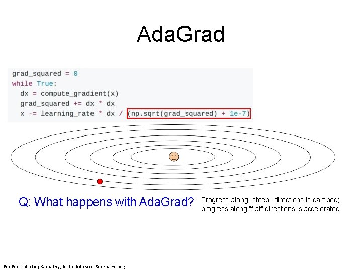
Ada. Grad Q: What happens with Ada. Grad? Fei-Fei Li & Justin Johnson & Serena Yeung Fei-Fei Li, Andrej Karpathy, Justin Johnson, Serena Yeung April 24, 2018 Progress along “steep” directions is damped; progress along “flat” directions is accelerated Lecture 7 - April 24, 2018

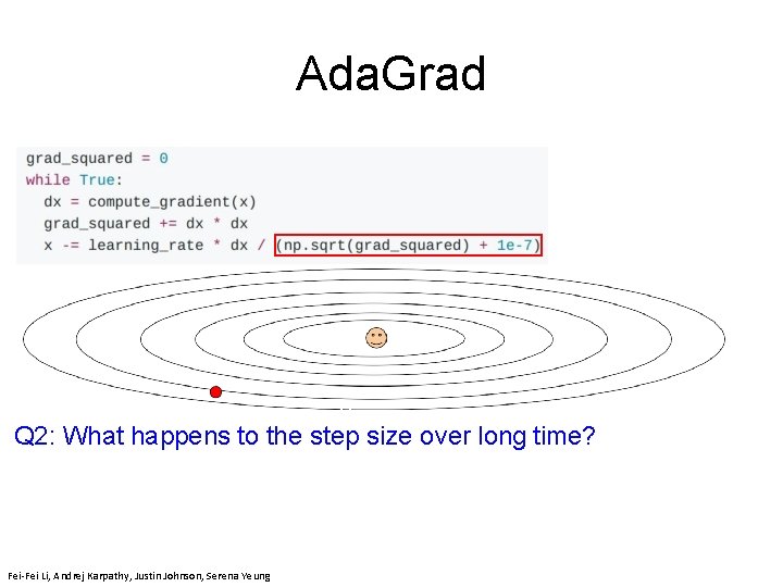
Ada. Grad Fei-Fei Li & Justin Johnson & Serena Yeung Q 2: What happens to the step size over long time? Fei-Fei Li & Justin Johnson & Serena Yeung Fei-Fei Li, Andrej Karpathy, Justin Johnson, Serena Yeung Lecture 7 - April 24, 2018

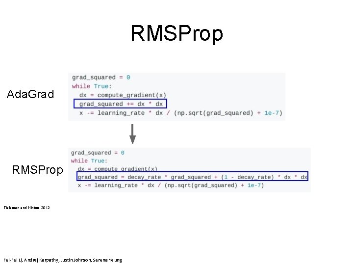
RMSProp Ada. Grad RMSProp Tieleman and Hinton, 2012 Fei-Fei Li & Justin Johnson & Serena Yeung Fei-Fei Li, Andrej Karpathy, Justin Johnson, Serena Yeung Lecture 7 - April 24, 2018

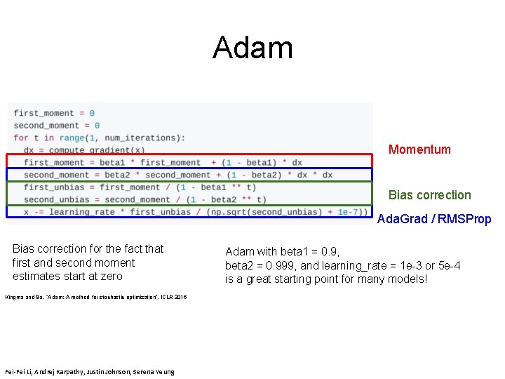
Adam Momentum Bias correction Ada. Grad / RMSProp Bias correction for the fact that Adam with beta 1 = 0. 9, first and second moment beta 2 = 0. 999, Lecture and learning_rate = 1 e-3 or 5 e-4 Fei-Fei Li & Justin Johnson & Serena Yeung April 24, 2018 7 86 estimates start at zero is a great starting point for many models! Kingma and Ba, “Adam: A method for stochastic optimization”, ICLR 2015 Fei-Fei Li & Justin Johnson & Serena Yeung Fei-Fei Li, Andrej Karpathy, Justin Johnson, Serena Yeung Lecture 7 - April 24, 2018

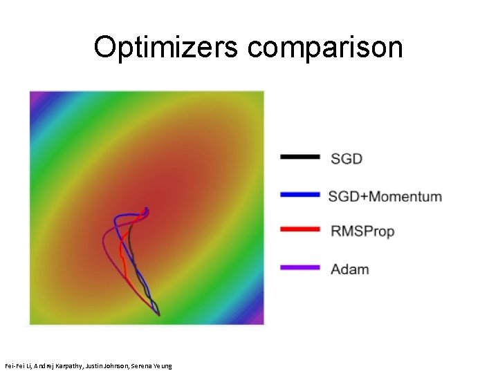
Optimizers comparison Fei-Fei Li, Andrej Karpathy, Justin Johnson, Serena Yeung

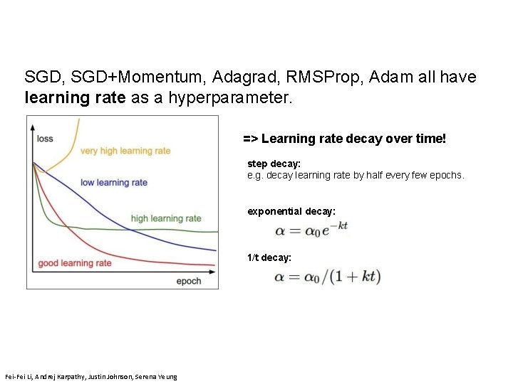
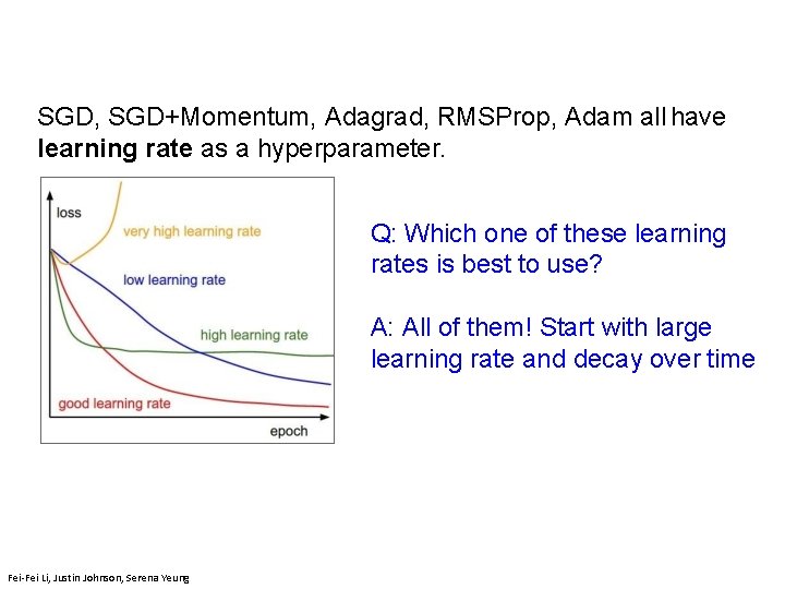
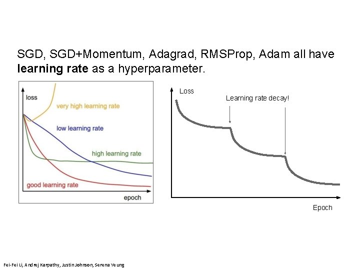
SGD, SGD+Momentum, Adagrad, RMSProp, Adam all have learning rate as a hyperparameter. => Learning rate decay over time! step decay: e. g. decay learning rate by half every few epochs. exponential decay: 1/t decay: April 24, 2018 Fei-Fei Li & Justin Johnson & Serena Yeung Fei-Fei Li, Andrej Karpathy, Justin Johnson, Serena Yeung Lecture 7 - April 24, 2018

SGD, SGD+Momentum, Adagrad, RMSProp, Adam all have learning rate as a hyperparameter. Q: Which one of these learning rates is best to use? A: All of them! Start with large learning rate and decay over time 89 April 25, 2019 Fei-Fei Li & Justin Johnson & Serena Yeung Fei-Fei Li, Justin Johnson, Serena Yeung Lecture 7 - April 24, 2018

SGD, SGD+Momentum, Adagrad, RMSProp, Adam all have learning rate as a hyperparameter. Loss Learning rate decay! Lecture 7 - 90 April 24, 2018 Epoch Fei-Fei Li & Justin Johnson & Serena Yeung Fei-Fei Li, Andrej Karpathy, Justin Johnson, Serena Yeung Lecture 7 - April 24, 2018

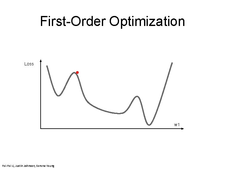
First-Order Optimization Loss 91 April 25, 2019 w 1 Fei-Fei Li & Justin Johnson & Serena Yeung Fei-Fei Li, Justin Johnson, Serena Yeung Lecture 7 - April 24, 2018

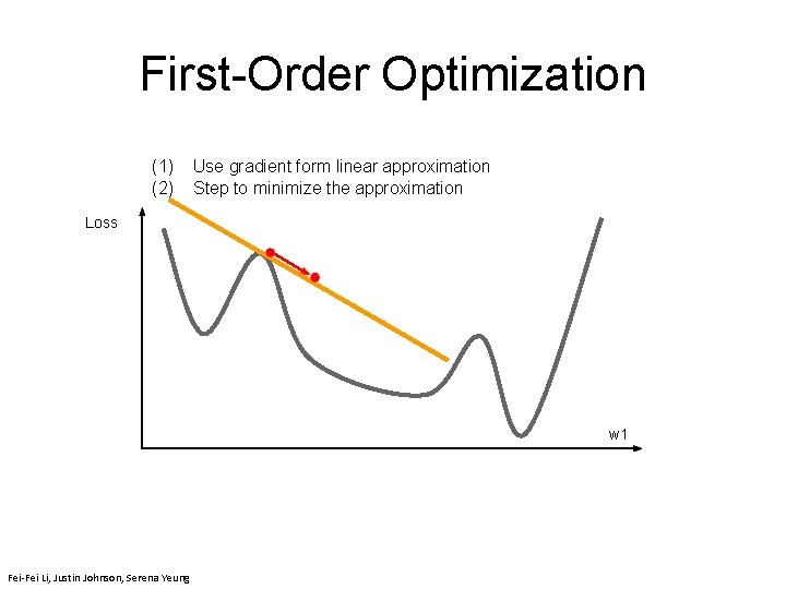
First-Order Optimization (1) (2) Use gradient form linear approximation Step to minimize the approximation Loss 92 April 25, 2019 w 1 Fei-Fei Li & Justin Johnson & Serena Yeung Fei-Fei Li, Justin Johnson, Serena Yeung Lecture 7 - April 24, 2018

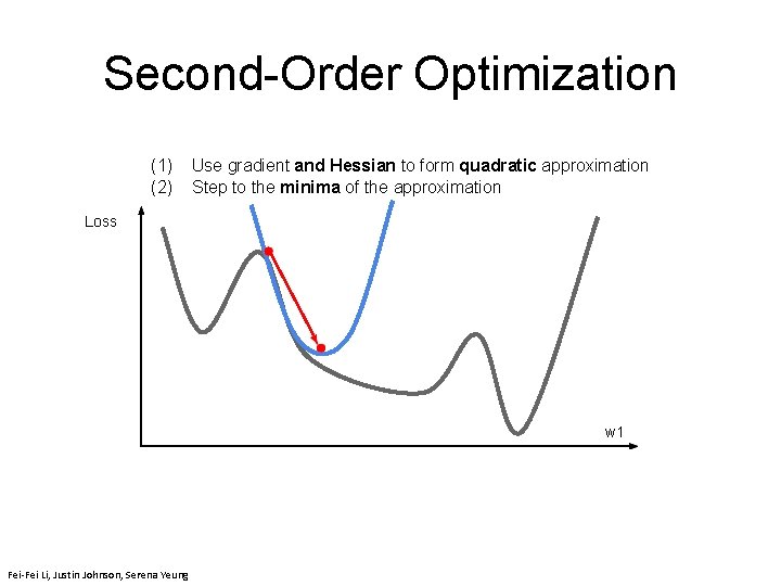
Second-Order Optimization (1) (2) Use gradient and Hessian to form quadratic approximation Step to the minima of the approximation Loss 93 April 25, 2019 w 1 Fei-Fei Li & Justin Johnson & Serena Yeung Fei-Fei Li, Justin Johnson, Serena Yeung Lecture 7 - April 24, 2018

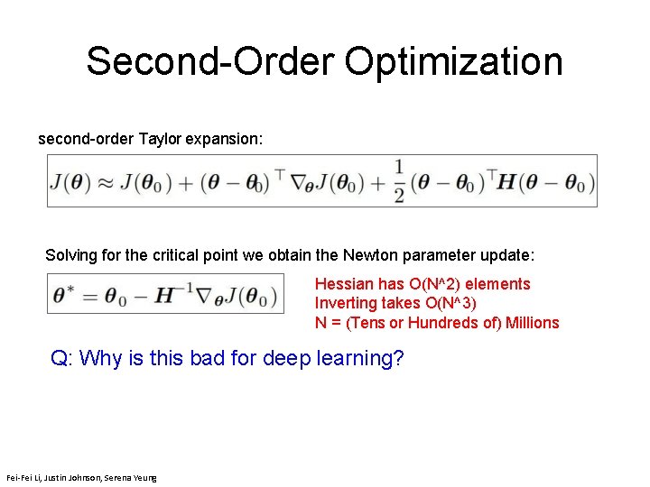
Second-Order Optimization second-order Taylor expansion: Solving for the critical point we obtain the Newton parameter update: Hessian has O(N^2) elements Inverting takes O(N^3) N = (Tens or Hundreds of) Millions Fei-Fei Li & Justin Johnson & Serena Yeung 94 April 25, 2019 Q: Why is this bad for deep learning? Fei-Fei Li & Justin Johnson & Serena Yeung Fei-Fei Li, Justin Johnson, Serena Yeung Lecture 7 - April 24, 2018

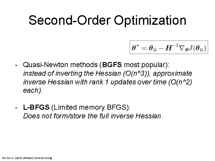
Second-Order Optimization - Quasi-Newton methods (BGFS most popular): instead of inverting the Hessian (O(n^3)), approximate inverse Hessian with rank 1 updates over time (O(n^2) each). - L-BFGS (Limited memory BFGS): Does not form/store the full inverse Hessian. 95 April 25, 2019 Fei-Fei Li & Justin Johnson & Serena Yeung Fei-Fei Li, Justin Johnson, Serena Yeung Lecture 7 - April 24, 2018

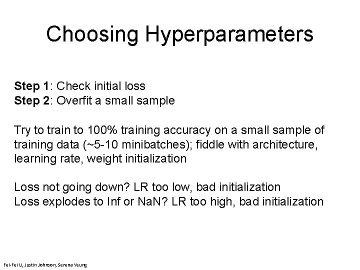
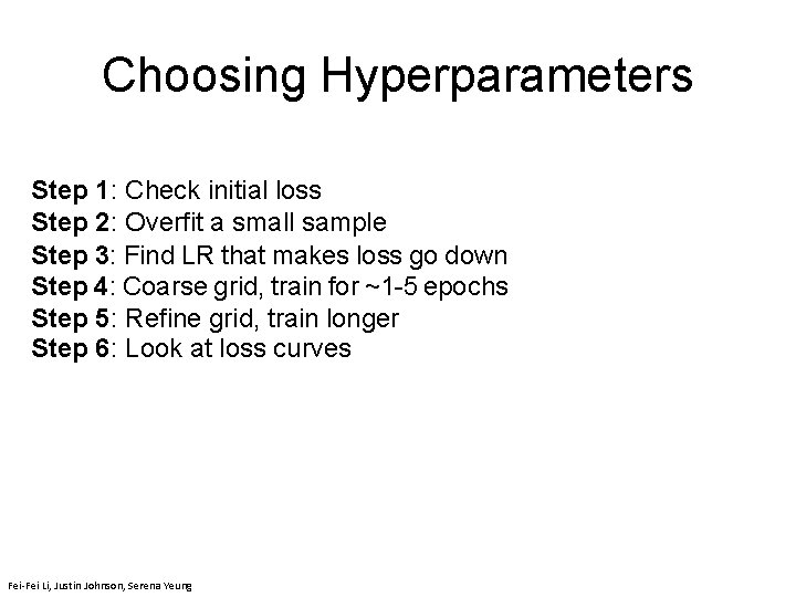
Choosing Hyperparameters Step 1: Check initial loss Turn off weight decay, sanity check loss at initialization e. g. log(C) for softmax with C classes 96 April 25, 2019 Fei-Fei Li & Justin Johnson & Serena Yeung Fei-Fei Li, Justin Johnson, Serena Yeung Lecture 7 - April 24, 2018

Choosing Hyperparameters Step 1: Check initial loss Step 2: Overfit a small sample Try to train to 100% training accuracy on a small sample of training data (~5 -10 minibatches); fiddle with architecture, learning rate, weight initialization Loss. Linot going down? LR too low, Fei-Fei & Justin Johnson & Serena Yeung bad initialization 97 April 25, 2019 Loss explodes to Inf or Na. N? LR too high, bad initialization Fei-Fei Li & Justin Johnson & Serena Yeung Fei-Fei Li, Justin Johnson, Serena Yeung Lecture 7 - April 24, 2018

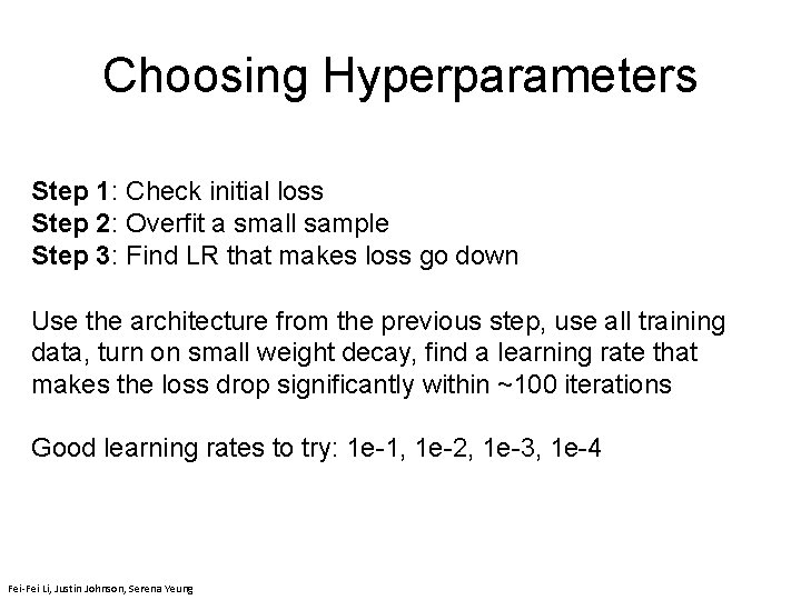
Choosing Hyperparameters Step 1: Check initial loss Step 2: Overfit a small sample Step 3: Find LR that makes loss go down Use the architecture from the previous step, use all training data, turn on small weight decay, find a learning rate that makes the loss drop significantly within ~100 iterations Fei-Fei Li & Justin Johnson & Serena Yeung Good learning rates to try: 1 e-1, 1 e-2, 1 e-3, 1 e-4 Fei-Fei Li & Justin Johnson & Serena Yeung Fei-Fei Li, Justin Johnson, Serena Yeung Lecture 7 - 98 April 25, 2019 April 24, 2018

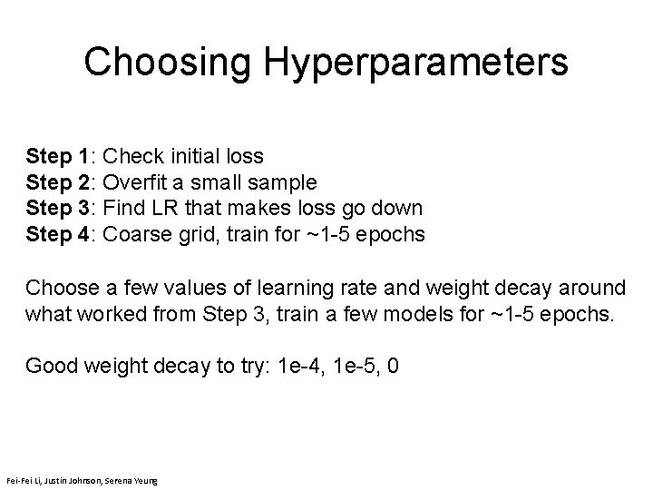
Choosing Hyperparameters Step 1: Check initial loss Step 2: Overfit a small sample Step 3: Find LR that makes loss go down Step 4: Coarse grid, train for ~1 -5 epochs Choose a few values of learning rate and weight decay around what worked from Step 3, train a few models for ~1 -5 epochs. Fei-Fei Li & Justin Johnson & Serena Yeung Good weight decay to try: 1 e-4, 1 e-5, 0 Fei-Fei Li & Justin Johnson & Serena Yeung Fei-Fei Li, Justin Johnson, Serena Yeung Lecture 7 - 99 April 25, 2019 April 24, 2018

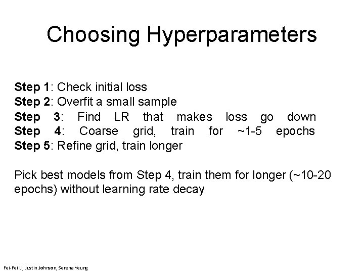
Choosing Hyperparameters Step 1: Check initial loss Step 2: Overfit a small sample Step 3: Find LR that makes loss go down Step 4: Coarse grid, train for ~1 -5 epochs Step 5: Refine grid, train longer Pick best models from Step 4, train them for longer (~10 -20 epochs) without learning rate decay Fei-Fei Li & Justin Johnson & Serena Yeung 10 April 25, 2019 0 Fei-Fei Li & Justin Johnson & Serena Yeung Fei-Fei Li, Justin Johnson, Serena Yeung Lecture 7 - April 24, 2018

Choosing Hyperparameters Step 1: Check initial loss Step 2: Overfit a small sample Step 3: Find LR that makes loss go down Step 4: Coarse grid, train for ~1 -5 epochs Step 5: Refine grid, train longer Step 6: Look at loss curves 10 April 25, 2019 1 Fei-Fei Li & Justin Johnson & Serena Yeung Fei-Fei Li, Justin Johnson, Serena Yeung Lecture 7 - April 24, 2018

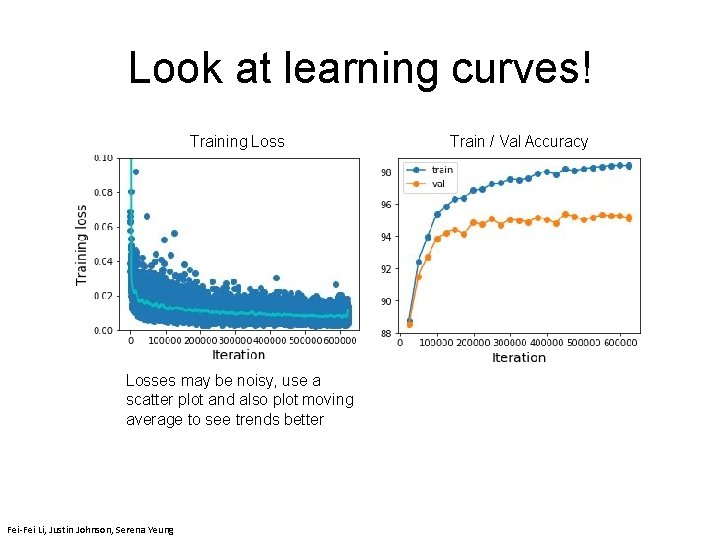
Look at learning curves! Training Loss Train / Val Accuracy 10 April 25, 2019 2 Losses may be noisy, use a scatter plot and also plot moving average to see trends better Fei-Fei Li & Justin Johnson & Serena Yeung Fei-Fei Li, Justin Johnson, Serena Yeung Lecture 7 - April 24, 2018

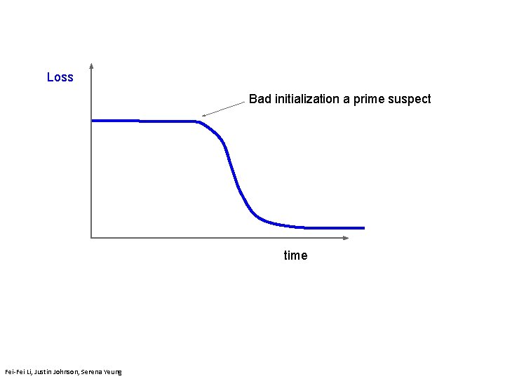
Loss Bad initialization a prime suspect Fei-Fei Li & Justin Johnson & Serena Yeung Fei-Fei Li, Justin Johnson, Serena Yeung time Lecture 7 - 10 April 25, 2019 3 April 24, 2018

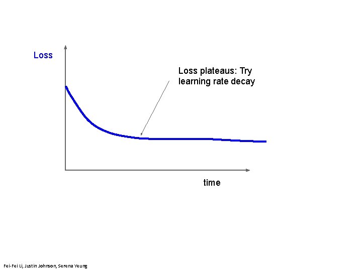
Loss plateaus: Try learning rate decay Fei-Fei Li & Justin Johnson & Serena Yeung Fei-Fei Li, Justin Johnson, Serena Yeung time Lecture 7 - 104 April 25, 2019

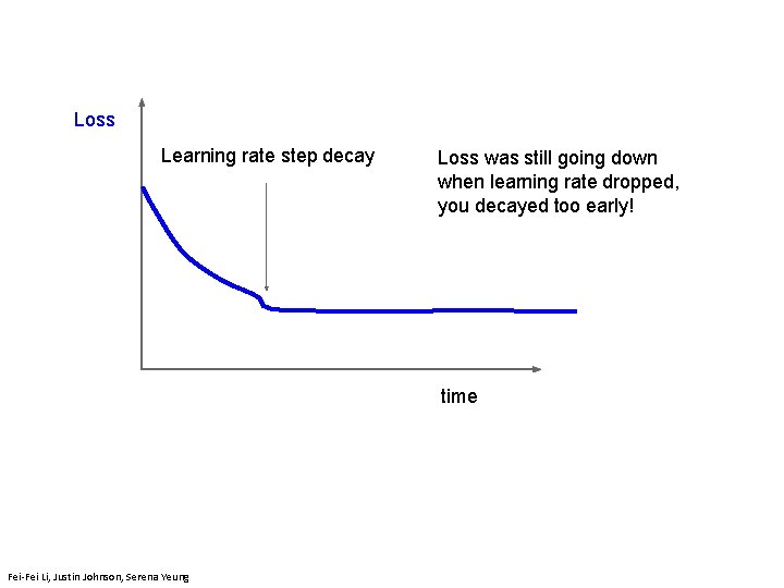
Loss Learning rate step decay Loss was still going down when learning rate dropped, you decayed too early! time Fei-Fei Li & Justin Johnson & Serena Yeung Fei-Fei Li, Justin Johnson, Serena Yeung Lecture 7 - 105 April 25, 2019

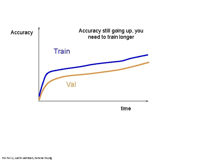
Accuracy still going up, you need to train longer Accuracy Train Val Fei-Fei Li & Justin Johnson & Serena Yeung Fei-Fei Li, Justin Johnson, Serena Yeung time Lecture 7 - 106 April 25, 2019

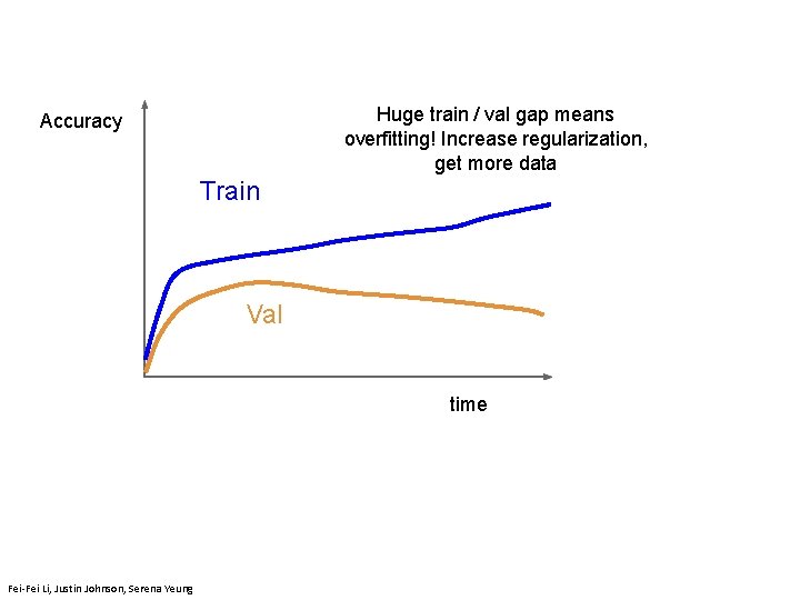
Huge train / val gap means overfitting! Increase regularization, get more data Accuracy Train Val Fei-Fei Li & Justin Johnson & Serena Yeung Fei-Fei Li, Justin Johnson, Serena Yeung time Lecture 7 - 107 April 25, 2019

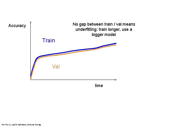
No gap between train / val means underfitting: train longer, use a bigger model Accuracy Train Val Fei-Fei Li & Justin Johnson & Serena Yeung Fei-Fei Li, Justin Johnson, Serena Yeung time Lecture 7 - 108 April 25, 2019

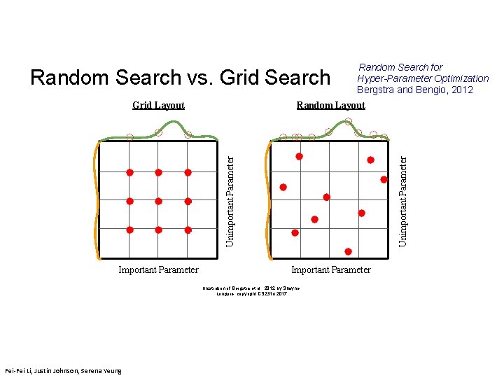
Random Search vs. Grid Search Unimportant Parameter Random Layout Unimportant Parameter Grid Layout Random Search for Hyper-Parameter Optimization Bergstra and Bengio, 2012 Important Parameter April 25, 2019 Illustration of Bergstra et al. , 2012 by Shayne Longpre, copyright CS 231 n 2017 Fei-Fei Li & Justin Johnson & Serena Yeung Fei-Fei Li, Justin Johnson, Serena Yeung Lecture 7 - 109 April 25, 2019

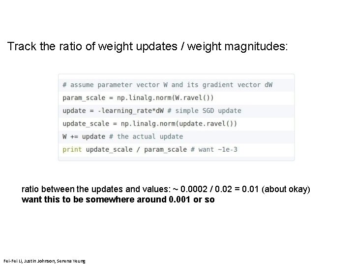
Track the ratio of weight updates / weight magnitudes: ratio between the updates and values: ~ 0. 0002 / 0. 02 = 0. 01 (about okay) want this to be somewhere around 0. 001 or so Fei-Fei Li & Justin Johnson & Serena Yeung Fei-Fei Li, Justin Johnson, Serena Yeung Lecture 7 - 110 April 25, 2019

Mini batch size Bhiksha Raj; Goyal et al. “Accurate, Large Minibatch SGD: Training Image. Net in 1 Hour”

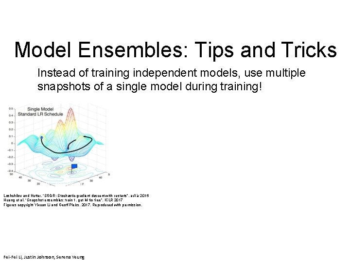
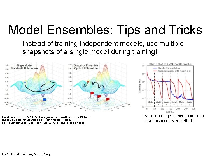
Model Ensembles 1. Train multiple independent models 2. At test time average their results (Take average of predicted probability distributions, then choose argmax) Enjoy 2% extra performance 11 April 25, 2019 2 Fei-Fei Li & Justin Johnson & Serena Yeung Fei-Fei Li, Justin Johnson, Serena Yeung Lecture 7 - April 24, 2018

Model Ensembles: Tips and Tricks Instead of training independent models, use multiple snapshots of a single model during training! 11 April 25, 2019 3 Fei-Fei Li & Justin Johnson & Serena Yeung Loshchilov and Hutter, “SGDR: Stochastic gradient descent with restarts”, ar. Xiv 2016 Huang et al, “Snapshot ensembles: train 1, get M for free”, ICLR 2017 Figures copyright Yixuan Li and Geoff Pleiss, 2017. Reproduced with permission. Fei-Fei Li & Justin Johnson & Serena Yeung Fei-Fei Li, Justin Johnson, Serena Yeung Lecture 7 - April 24, 2018

Model Ensembles: Tips and Tricks Instead of training independent models, use multiple snapshots of a single model during training! Fei-Fei Li & Justin Johnson & Serena Yeung Loshchilov and Hutter, “SGDR: Stochastic gradient descent with restarts”, ar. Xiv 2016 Huang et al, “Snapshot ensembles: train 1, get M for free”, ICLR 2017 Figures copyright Yixuan Li and Geoff Pleiss, 2017. Reproduced with permission. Fei-Fei Li & Justin Johnson & Serena Yeung Fei-Fei Li, Justin Johnson, Serena Yeung April 25, 2019 Cyclic learning rate schedules can make this work even better! Lecture 7 - 58 April 24, 2018

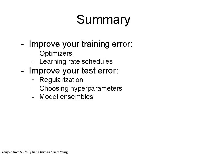
Summary - Improve your training error: - Optimizers - Learning rate schedules - Improve your test error: - Regularization - Choosing hyperparameters - Model ensembles April 25, 2019 Fei-Fei Li & Justin Johnson & Serena Yeung Adapted from Fei-Fei Li, Justin Johnson, Serena Yeung Lecture 7 - 115 April 25, 2019

Computation graphs

How do we compute the gradient? • Derive on paper? Tedious • What about vector-valued functions?

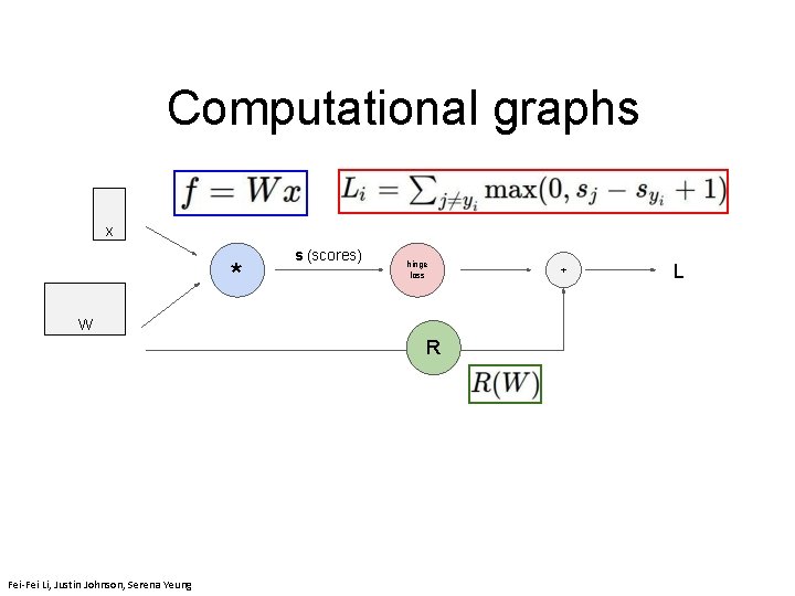
Computational graphs x * s (scores) hinge loss + L W R Fei-Fei Li & Justin Johnson & Serena Yeung Fei-Fei Li, Justin Johnson, Serena Yeung Lecture 4 118 April 11, 2019

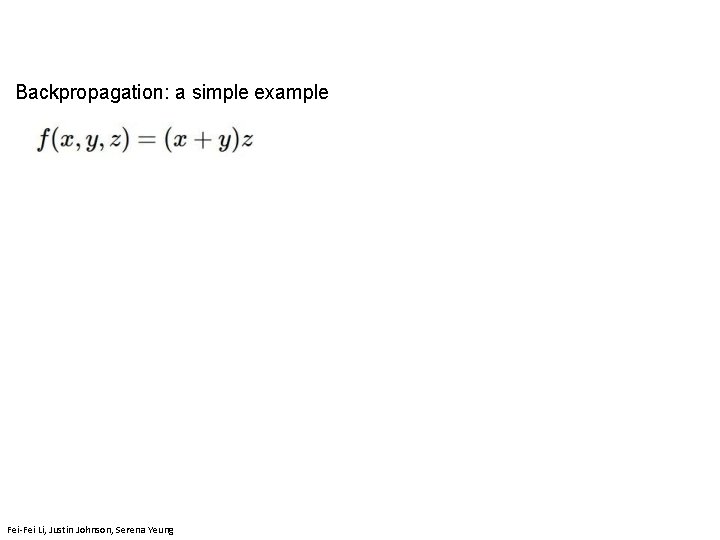
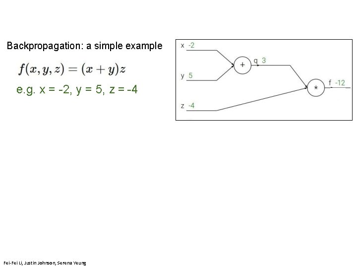
Backpropagation: a simple example Fei-Fei Li & Justin Johnson & Serena Yeung Fei-Fei Li, Justin Johnson, Serena Yeung Lecture 4 119 April 11, 2019

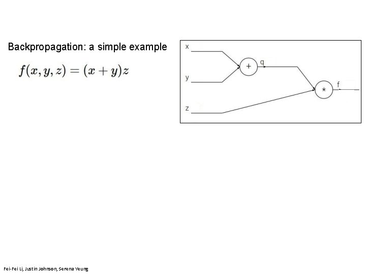
Backpropagation: a simple example Fei-Fei Li & Justin Johnson & Serena Yeung Fei-Fei Li, Justin Johnson, Serena Yeung Lecture 4 120 April 11, 2019

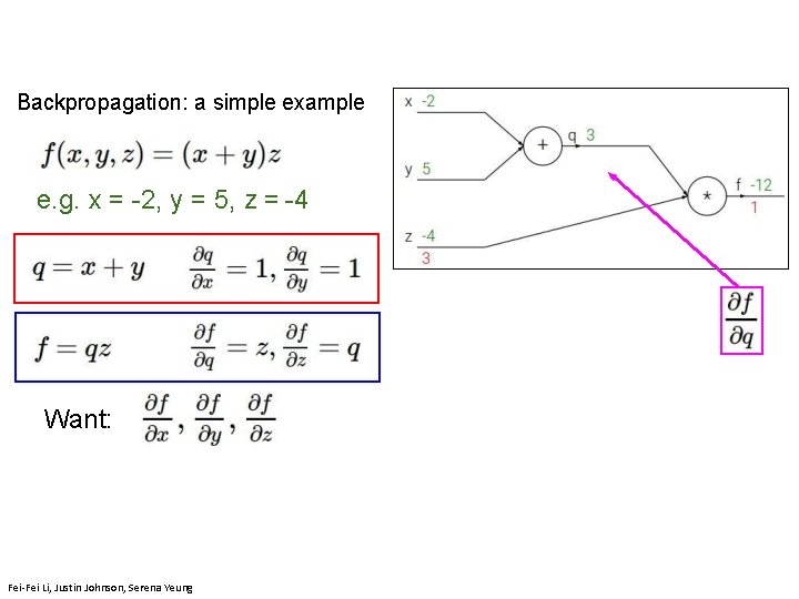
Backpropagation: a simple example e. g. x = -2, y = 5, z = -4 Fei-Fei Li, Justin Johnson, Serena Yeung

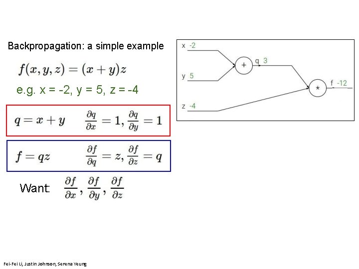
Backpropagation: a simple example e. g. x = -2, y = 5, z = -4 Want: Fei-Fei Li, Justin Johnson, Serena Yeung Lecture 4 122 April 11, 2019

Backpropagation: a simple example e. g. x = -2, y = 5, z = -4 Want: Fei-Fei Li, Justin Johnson, Serena Yeung Lecture 4 123 April 11, 2019

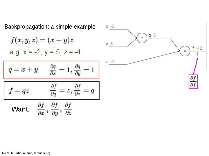
Backpropagation: a simple example e. g. x = -2, y = 5, z = -4 Want: Fei-Fei Li, Justin Johnson, Serena Yeung Lecture 4 124 April 11, 2019

Backpropagation: a simple example e. g. x = -2, y = 5, z = -4 Want: Fei-Fei Li, Justin Johnson, Serena Yeung Lecture 4 125 April 11, 2019

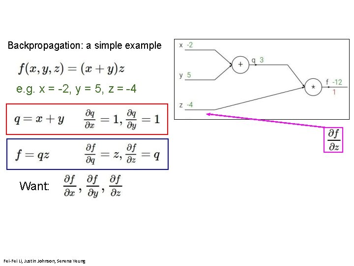
Backpropagation: a simple example e. g. x = -2, y = 5, z = -4 Want: Fei-Fei Li, Justin Johnson, Serena Yeung Lecture 4 126 April 11, 2019

Backpropagation: a simple example e. g. x = -2, y = 5, z = -4 Want: Fei-Fei Li, Justin Johnson, Serena Yeung Lecture 4 127 April 11, 2019

Backpropagation: a simple example e. g. x = -2, y = 5, z = -4 Want: Fei-Fei Li, Justin Johnson, Serena Yeung Lecture 4 128 April 11, 2019

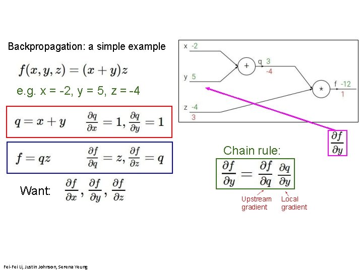
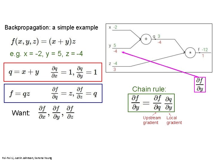
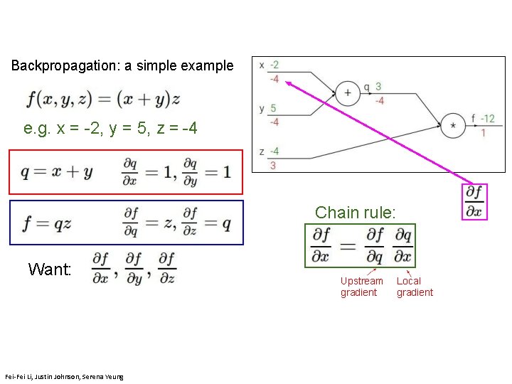
Backpropagation: a simple example e. g. x = -2, y = 5, z = -4 Chain rule: Want: Upstream gradient Local gradient April 13, 2017 Fei-Fei Li, Justin Johnson, Serena Yeung

Backpropagation: a simple example e. g. x = -2, y = 5, z = -4 Chain rule: Want: Upstream gradient Local gradient April 13, 2017 Fei-Fei Li, Justin Johnson, Serena Yeung

Backpropagation: a simple example e. g. x = -2, y = 5, z = -4 Chain rule: Want: Upstream gradient Local gradient April 13, 2017 Fei-Fei Li, Justin Johnson, Serena Yeung

Backpropagation: a simple example e. g. x = -2, y = 5, z = -4 Chain rule: Want: Upstream gradient Local gradient April 13, 2017 Fei-Fei Li, Justin Johnson, Serena Yeung

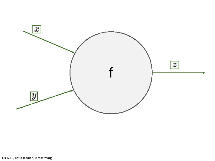
f April 11, 2019 Fei-Fei Li, Justin Johnson, Serena Yeung

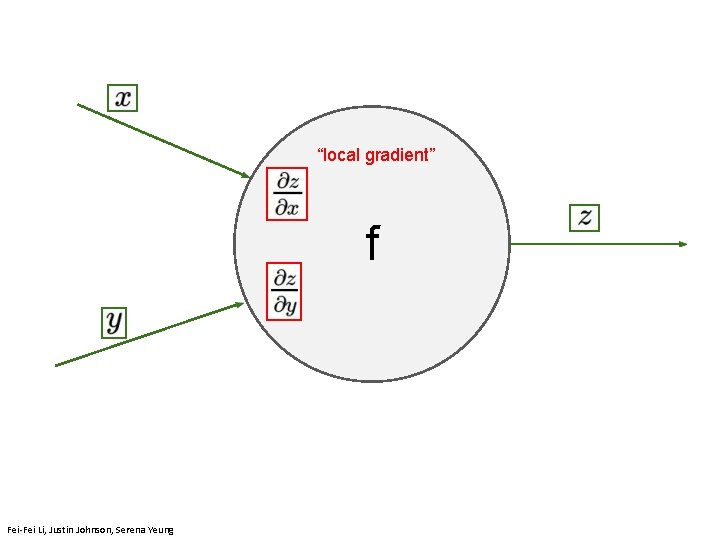
“local gradient” f April 11, 2019 Fei-Fei Li, Justin Johnson, Serena Yeung

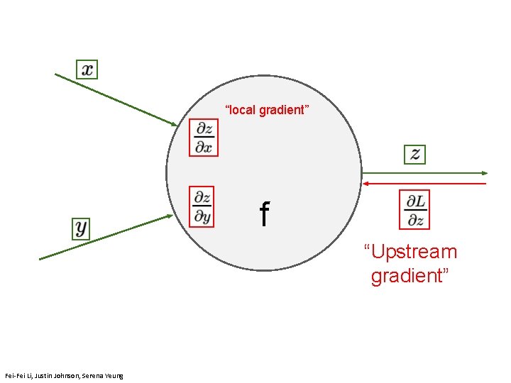
“local gradient” f “Upstream gradient” Fei-Fei Li, Justin Johnson, Serena Yeung

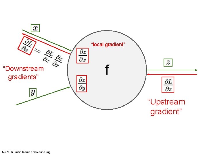
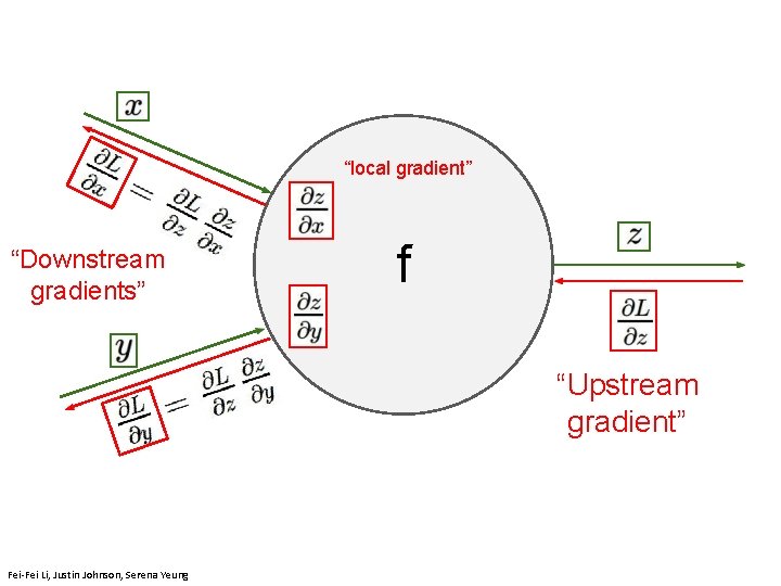
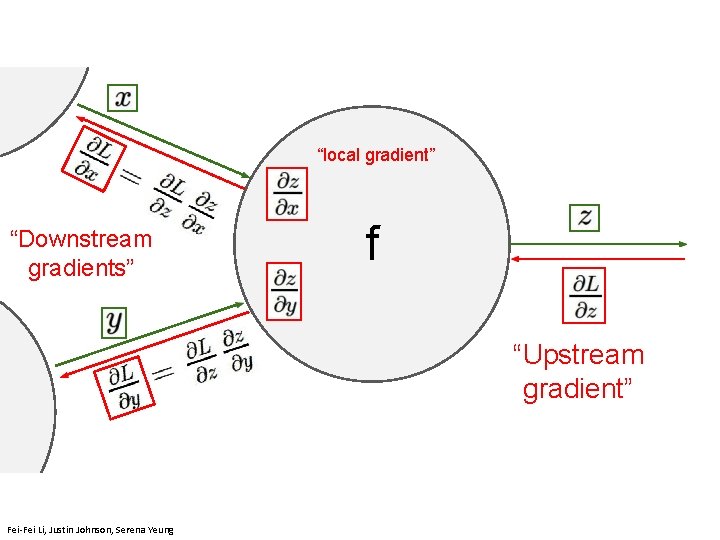
“local gradient” “Downstream gradients” f “Upstream April 11, 2019 gradient” Fei-Fei Li, Justin Johnson, Serena Yeung

“local gradient” “Downstream gradients” f “Upstream April 11, 2019 gradient” Fei-Fei Li, Justin Johnson, Serena Yeung

“local gradient” “Downstream gradients” f “Upstream April 11, 2019 gradient” Fei-Fei Li, Justin Johnson, Serena Yeung

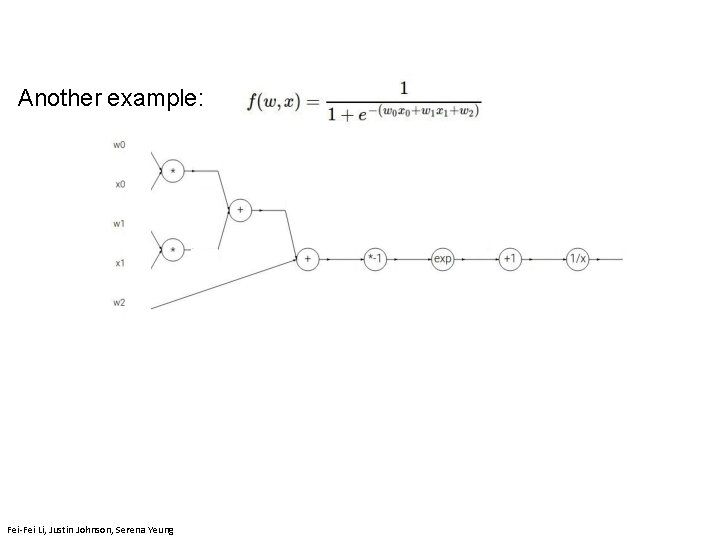
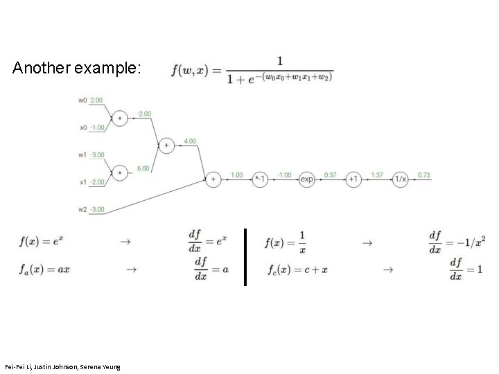
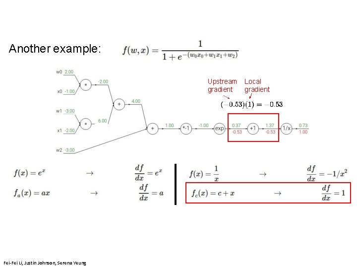
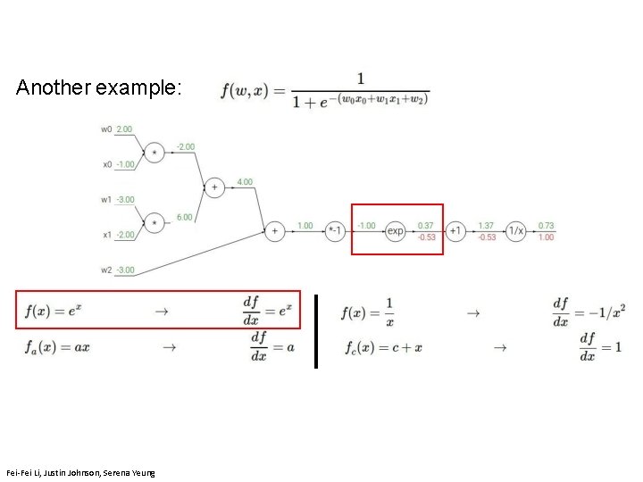
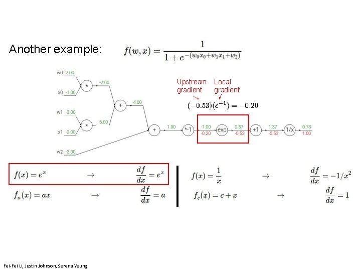
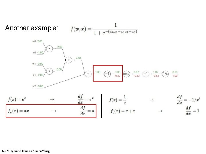
Another example: Fei-Fei Li & Justin Johnson & Serena Yeung Fei-Fei Li, Justin Johnson, Serena Yeung Lecture 4 139 April 11, 2019

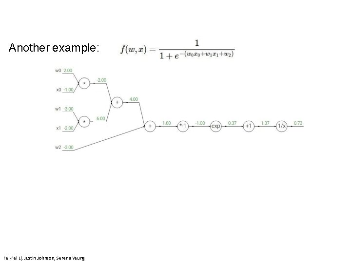
Another example: Fei-Fei Li & Justin Johnson & Serena Yeung Fei-Fei Li, Justin Johnson, Serena Yeung Lecture 4 140 April 11, 2019

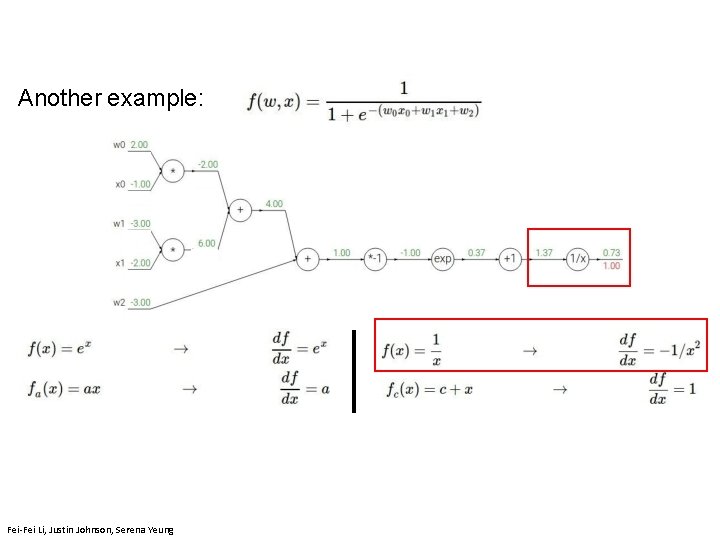
Another example: Fei-Fei Li, Justin Johnson, Serena Yeung

Another example: Fei-Fei Li, Justin Johnson, Serena Yeung

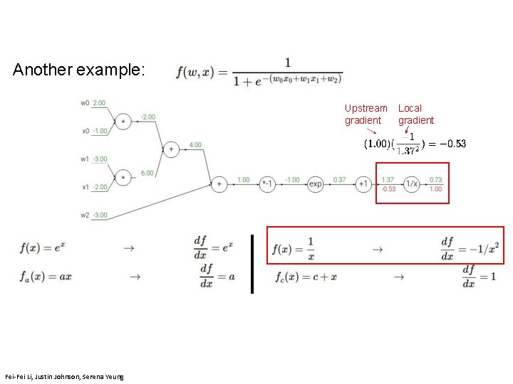
Another example: Upstream gradient Fei-Fei Li, Justin Johnson, Serena Yeung Local gradient

Another example: Fei-Fei Li, Justin Johnson, Serena Yeung

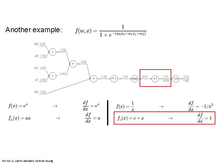
Another example: Upstream gradient Fei-Fei Li, Justin Johnson, Serena Yeung Local gradient

Another example: Fei-Fei Li, Justin Johnson, Serena Yeung

Another example: Upstream gradient Fei-Fei Li, Justin Johnson, Serena Yeung Local gradient

Another example: Fei-Fei Li, Justin Johnson, Serena Yeung

Another example: Upstream gradient Fei-Fei Li, Justin Johnson, Serena Yeung Local gradient

Another example: Fei-Fei Li, Justin Johnson, Serena Yeung
![Another example upstream gradient x local gradient 0 2 x 1 0 2 Another example: [upstream gradient] x [local gradient] [0. 2] x [1] = 0. 2](https://slidetodoc.com/presentation_image_h2/9895368f71e9327388947d823a2357bc/image-151.jpg)
Another example: [upstream gradient] x [local gradient] [0. 2] x [1] = 0. 2 (both inputs!) Fei-Fei Li, Justin Johnson, Serena Yeung

Another example: Fei-Fei Li, Justin Johnson, Serena Yeung
![Another example upstream gradient x local gradient x 0 0 2 x 2 Another example: [upstream gradient] x [local gradient] x 0: [0. 2] x [2] =](https://slidetodoc.com/presentation_image_h2/9895368f71e9327388947d823a2357bc/image-153.jpg)
Another example: [upstream gradient] x [local gradient] x 0: [0. 2] x [2] = 0. 4 w 0: [0. 2] x [-1] = -0. 2 Fei-Fei Li, Justin Johnson, Serena Yeung

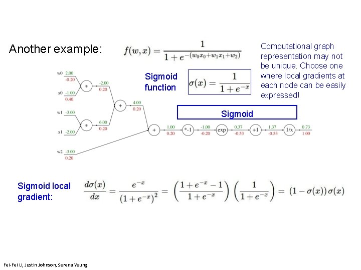
Computational graph representation may not be unique. Choose one where local gradients at each node can be easily expressed! Another example: Sigmoid function Sigmoid Fei-Fei Li & Justin Johnson & Serena Yeung Fei-Fei Li, Justin Johnson, Serena Yeung Lecture 4 154 April 11, 2019

Computational graph representation may not be unique. Choose one where local gradients at each node can be easily expressed! Another example: Sigmoid function Sigmoid local gradient: Fei-Fei Li, Justin Johnson, Serena Yeung

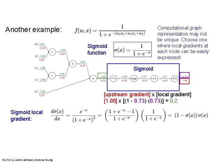
Computational graph representation may not be unique. Choose one where local gradients at each node can be easily expressed! Another example: Sigmoid function Sigmoid [upstream gradient] x [local gradient] [1. 00] x [(1 - 0. 73) (0. 73)] = 0. 2 Sigmoid local gradient: Fei-Fei Li, Justin Johnson, Serena Yeung

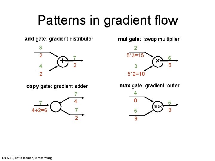
Patterns in gradient flow add gate: gradient distributor 3 2 4 2 + 7 2 copy gate: gradient adder 7 4+2=6 Fei-Fei Li, Justin Johnson, Serena Yeung 7 4 7 2 mul gate: “swap multiplier” 2 5*3=15 3 5*2=10 × 6 5 max gate: gradient router 4 0 5 5 9 max 9

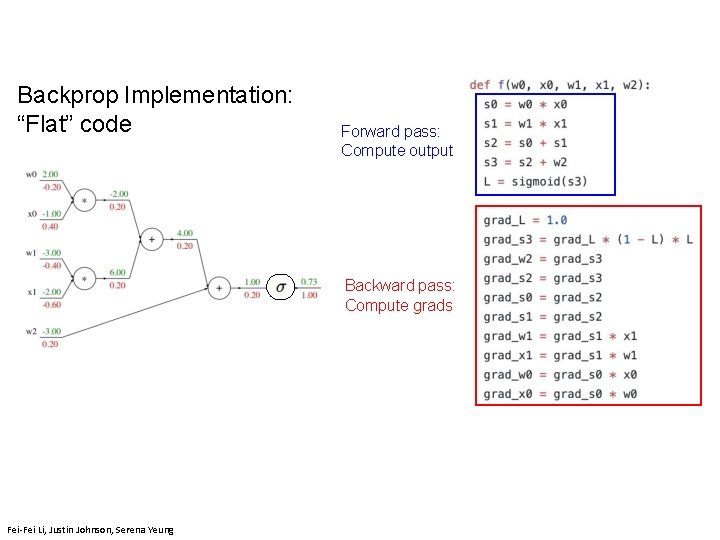
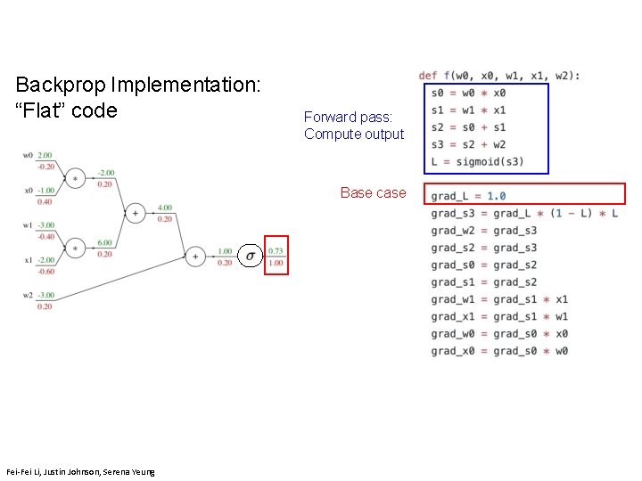
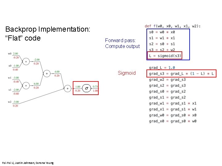
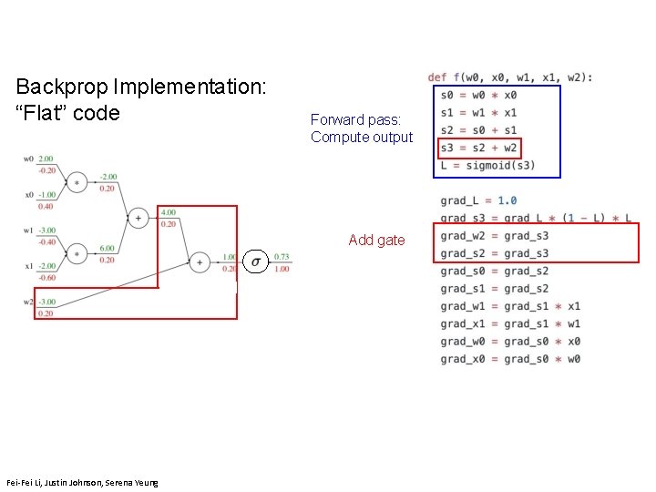
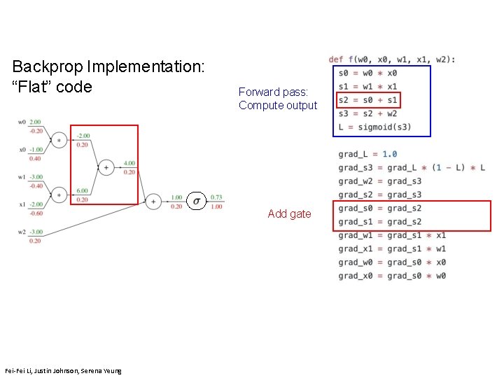
Backprop Implementation: “Flat” code Forward pass: Compute output Backward pass: Compute grads Fei-Fei Li, Justin Johnson, Serena Yeung

Backprop Implementation: “Flat” code Forward pass: Compute output Base case Fei-Fei Li, Justin Johnson, Serena Yeung

Backprop Implementation: “Flat” code Forward pass: Compute output Sigmoid Fei-Fei Li, Justin Johnson, Serena Yeung

Backprop Implementation: “Flat” code Forward pass: Compute output Add gate Fei-Fei Li, Justin Johnson, Serena Yeung

Backprop Implementation: “Flat” code Forward pass: Compute output Add gate Fei-Fei Li, Justin Johnson, Serena Yeung

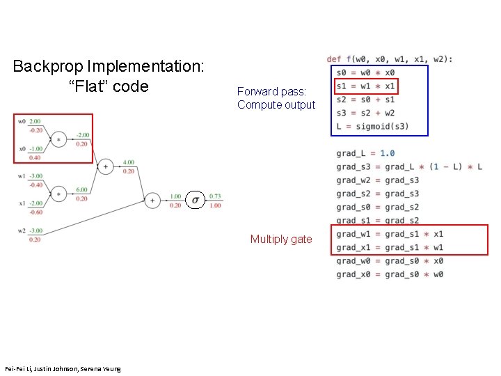
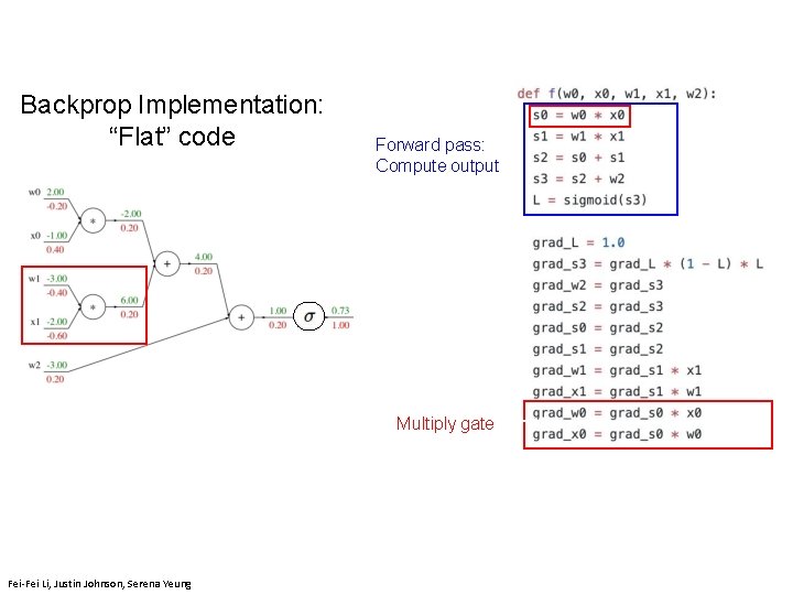
Backprop Implementation: “Flat” code Forward pass: Compute output Multiply gate Fei-Fei Li & Justin Johnson & Serena Yeung Fei-Fei Li, Justin Johnson, Serena Yeung Lecture 4 163

Backprop Implementation: “Flat” code Forward pass: Compute output Fei-Fei Li & Justin Johnson & Serena Yeung Multiply Lecture gate 4 164 Fei-Fei Li, Justin Johnson, Serena Yeung

So far: backprop with scalars What about vector-valued functions? Fei-Fei Li & Justin Johnson & Serena Yeung Fei-Fei Li, Justin Johnson, Serena Yeung Lecture 4 165 April 11, 2019

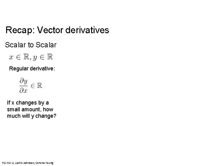
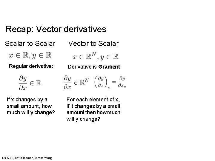
Recap: Vector derivatives Scalar to Scalar Regular derivative: If x changes by a small amount, how much will y change? April 11, 2019 Lecture 4 - 166 Fei-Fei Li, Justin Johnson, Serena Yeung

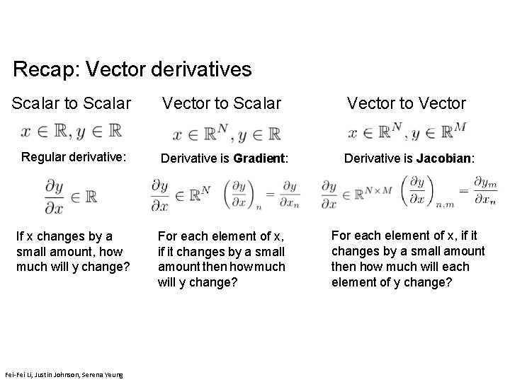
Recap: Vector derivatives Scalar to Scalar Vector to Scalar Regular derivative: Derivative is Gradient: If x changes by a small amount, how much will y change? For each element of x, if it changes by a small amount then how much will y change? April 11, 2019 Lecture 4 - 167 Fei-Fei Li, Justin Johnson, Serena Yeung

Recap: Vector derivatives Scalar to Scalar Vector to Vector Regular derivative: Derivative is Gradient: Derivative is Jacobian: If x changes by a small amount, how much will y change? For each element of x, if it changes by a small amount then how much will each element of y change? Lecture 4 - 168 Fei-Fei Li, Justin Johnson, Serena Yeung

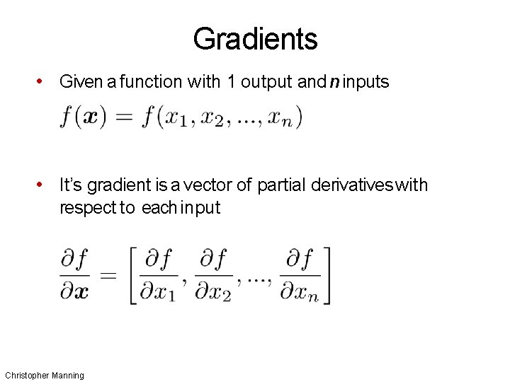
Gradients • Given a function with 1 output and n inputs • It’s gradient is a vector of partial derivatives with respect to each input Christopher Manning

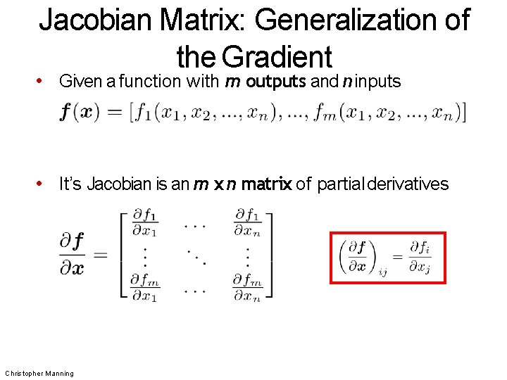
Jacobian Matrix: Generalization of the Gradient • Given a function with m outputs and n inputs • It’s Jacobian is an m x n matrix of partial derivatives Christopher Manning

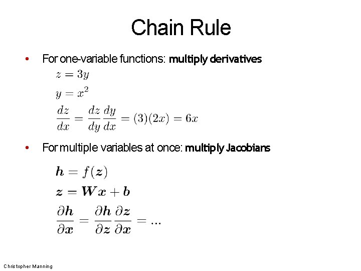
Chain Rule • For one-variable functions: multiply derivatives • For multiple variables at once: multiply. Jacobians Christopher Manning

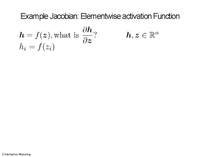
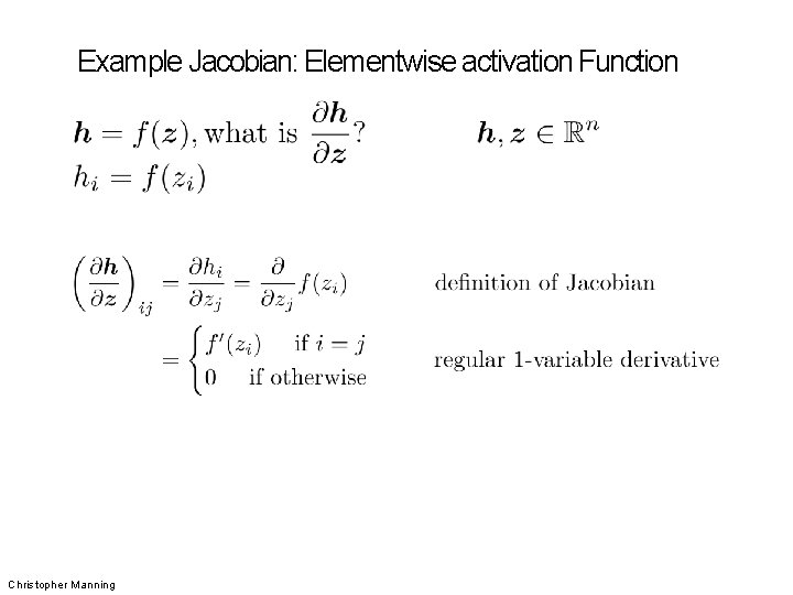
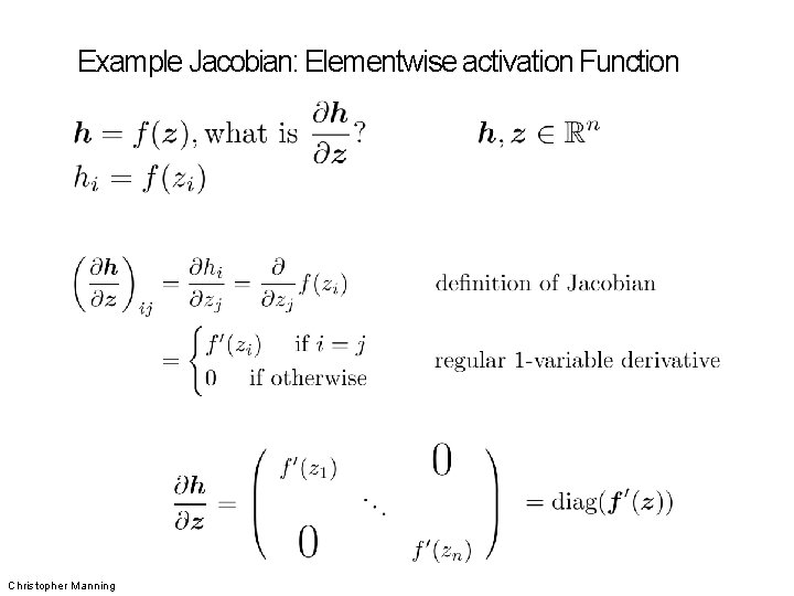
Example Jacobian: Elementwise activation Function Christopher Manning

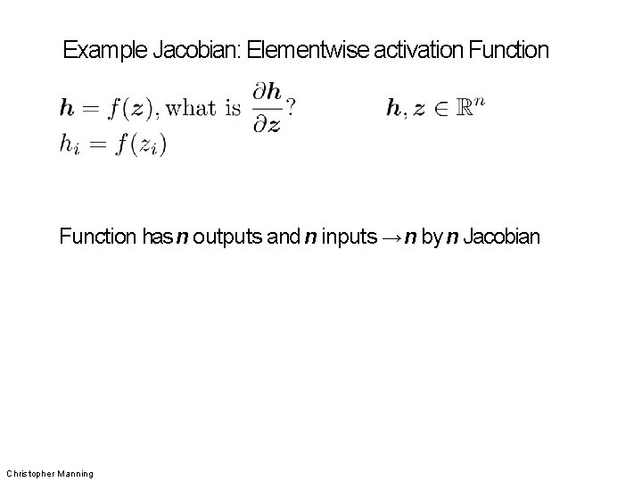
Example Jacobian: Elementwise activation Function has n outputs and n inputs → n by n Jacobian 173 Christopher Manning

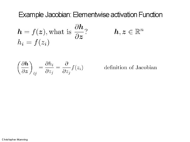
Example Jacobian: Elementwise activation Function Christopher Manning

Example Jacobian: Elementwise activation Function Christopher Manning

Example Jacobian: Elementwise activation Function Christopher Manning

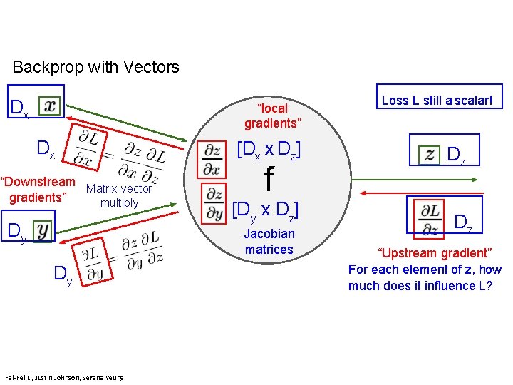
Backprop with Vectors Dx Loss L still a scalar! “local gradients” Dx “Downstream Matrix-vector gradients” multiply Dy [Dx x Dz] f [Dy x Dz] Jacobian matrices Dy Dz Dz “Upstream gradient” For each element of z, how much does it influence L? Lecture 4 - 177 Fei-Fei Li, Justin Johnson, Serena Yeung
![Backprop with Vectors 4 D input x 1 2 Backprop with Vectors 4 D input x: [ 1 ] [ -2 ] [](https://slidetodoc.com/presentation_image_h2/9895368f71e9327388947d823a2357bc/image-178.jpg)
Backprop with Vectors 4 D input x: [ 1 ] [ -2 ] [ 3 ] [ -1 ] f(x) = max(0, x) (elementwise) 4 D output y: [ 1 ] [ 0 ] [ 3 ] [ 0 ] Fei-Fei Li & Justin Johnson & Serena Yeung April 11, 2019 Lecture 4 - 178 Fei-Fei Li, Justin Johnson, Serena Yeung
![Backprop with Vectors 4 D input x 1 2 Backprop with Vectors 4 D input x: [ 1 ] [ -2 ] [](https://slidetodoc.com/presentation_image_h2/9895368f71e9327388947d823a2357bc/image-179.jpg)
Backprop with Vectors 4 D input x: [ 1 ] [ -2 ] [ 3 ] [ -1 ] f(x) = max(0, x) (elementwise) Fei-Fei Li & Justin Johnson & Serena Yeung 4 D output y: [ 1 ] [ 0 ] [ 3 ] [ 0 ] 4 D d. L/dy: [ 4 ] [ -1 ] [ 5 ] [ 9 ] Lecture 4 - 179 Fei-Fei Li, Justin Johnson, Serena Yeung Upstream gradient April 11, 2019
![Backprop with Vectors 4 D input x 1 2 Backprop with Vectors 4 D input x: [ 1 ] [ -2 ] [](https://slidetodoc.com/presentation_image_h2/9895368f71e9327388947d823a2357bc/image-180.jpg)
Backprop with Vectors 4 D input x: [ 1 ] [ -2 ] [ 3 ] [ -1 ] f(x) = max(0, x) (elementwise) Jacobian dy/dx [1000] [0010] [0000] 4 D output y: [ 1 ] [ 0 ] [ 3 ] [ 0 ] 4 D d. L/dy: [ 4 ] [ -1 ] [ 5 ] [ 9 ] Lecture 4 - 180 Fei-Fei Li, Justin Johnson, Serena Yeung Upstream gradient April 11, 2019
![Backprop with Vectors 4 D input x 1 2 Backprop with Vectors 4 D input x: [ 1 ] [ -2 ] [](https://slidetodoc.com/presentation_image_h2/9895368f71e9327388947d823a2357bc/image-181.jpg)
Backprop with Vectors 4 D input x: [ 1 ] [ -2 ] [ 3 ] [ -1 ] f(x) = max(0, x) (elementwise) [dy/dx] [d. L/dy] [1000][4 ] [ 0 0 ] [ -1 ] [0010][5 ] [0000][9 ] 4 D output y: [ 1 ] [ 0 ] [ 3 ] [ 0 ] 4 D d. L/dy: [ 4 ] [ -1 ] [ 5 ] [ 9 ] Lecture 4 - 181 Fei-Fei Li, Justin Johnson, Serena Yeung Upstream gradient April 11, 2019
![Backprop with Vectors 4 D input x 1 2 Backprop with Vectors 4 D input x: [ 1 ] [ -2 ] [](https://slidetodoc.com/presentation_image_h2/9895368f71e9327388947d823a2357bc/image-182.jpg)
Backprop with Vectors 4 D input x: [ 1 ] [ -2 ] [ 3 ] [ -1 ] 4 D d. L/dx: [4] [0] [5] [0] f(x) = max(0, x) (elementwise) [dy/dx] [d. L/dy] [1000][4 ] [ 0 0 ] [ -1 ] [0010][5 ] [0000][9 ] 4 D output y: [ 1 ] [ 0 ] [ 3 ] [ 0 ] 4 D d. L/dy: [ 4 ] [ -1 ] [ 5 ] [ 9 ] Lecture 4 - 182 Fei-Fei Li, Justin Johnson, Serena Yeung Upstream gradient April 11, 2019

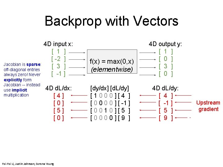
Backprop with Vectors Jacobian is sparse: off-diagonal entries always zero! Never explicitly form Jacobian -- instead use implicit multiplication 4 D input x: [ 1 ] [ -2 ] [ 3 ] [ -1 ] 4 D d. L/dx: [4] [0] [5] [0] f(x) = max(0, x) (elementwise) [dy/dx] [d. L/dy] [1000][4 ] [ 0 0 ] [ -1 ] [0010][5 ] [0000][9 ] 4 D output y: [ 1 ] [ 0 ] [ 3 ] [ 0 ] 4 D d. L/dy: [ 4 ] [ -1 ] [ 5 ] [ 9 ] Lecture 4 - 183 Fei-Fei Li, Justin Johnson, Serena Yeung Upstream gradient April 11, 2019
![Backprop with Matrices or Tensors DxMx local gradients DxMx DyMy d Ldx always has Backprop with Matrices (or Tensors) [Dx×Mx] “local gradients” [Dx×Mx] [Dy×My] d. L/dx always has](https://slidetodoc.com/presentation_image_h2/9895368f71e9327388947d823a2357bc/image-184.jpg)
Backprop with Matrices (or Tensors) [Dx×Mx] “local gradients” [Dx×Mx] [Dy×My] d. L/dx always has the same shape as x! [(Dx×Mx)×(Dz×Mz)] “Downstream Matrix-vector gradients” multiply [Dy×My] Loss L still a scalar! [Dz×Mz] [(Dy×My)×(Dz×Mz)] Jacobian matrices For each element of y, how much does it influence each element of z? [Dz×Mz] “Upstream gradient” For each element of z, how much does it influence L? Lecture 4 - 184 Fei-Fei Li, Justin Johnson, Serena Yeung

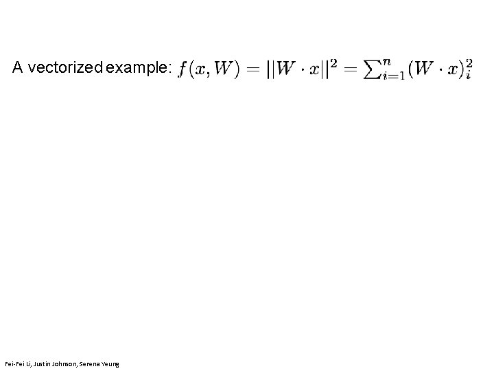
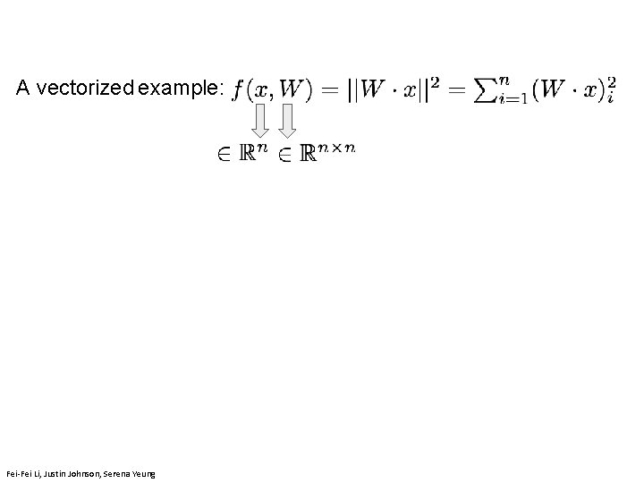
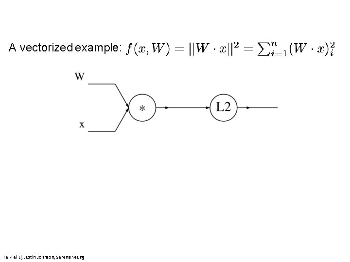
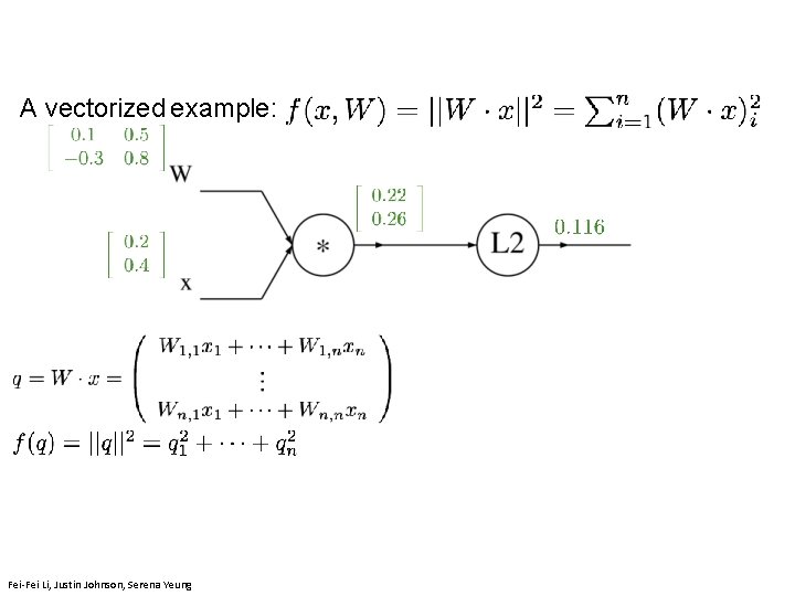
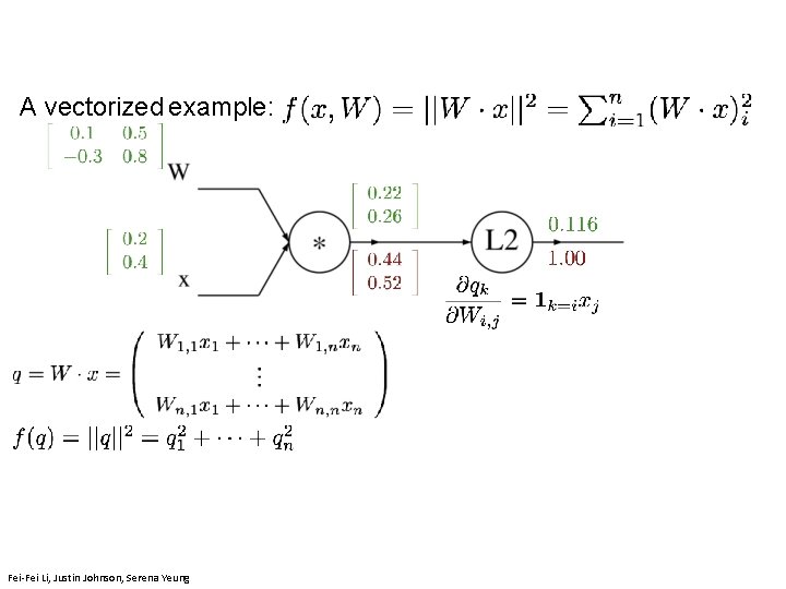
A vectorized example: Fei-Fei Li & Justin Johnson & Serena Yeung April 11, 2019 Lecture 4 - 185 Fei-Fei Li, Justin Johnson, Serena Yeung

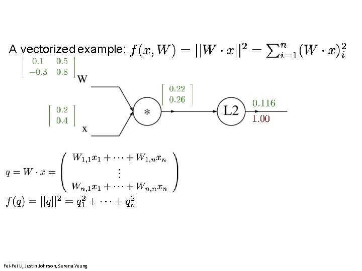
A vectorized example: Fei-Fei Li & Justin Johnson & Serena Yeung April 11, 2019 Lecture 4 - 186 Fei-Fei Li, Justin Johnson, Serena Yeung

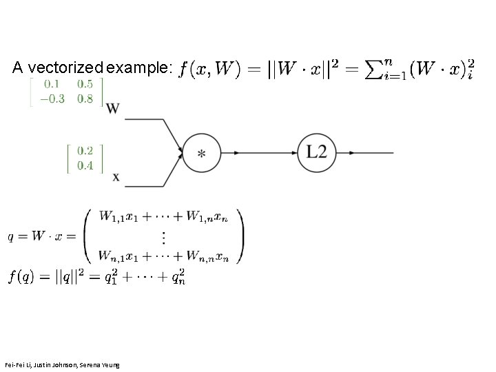
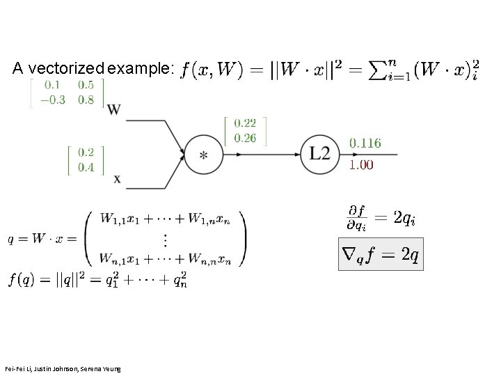
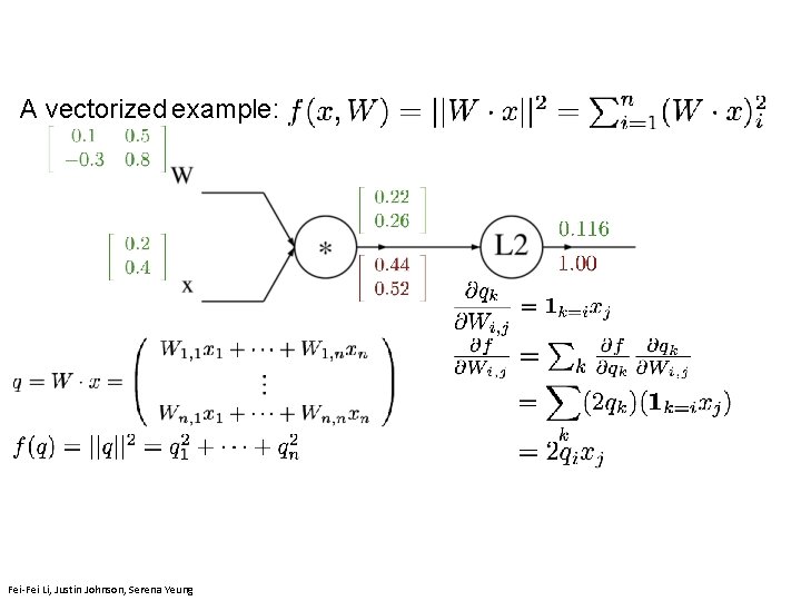
A vectorized example: Fei-Fei Li & Justin Johnson & Serena Yeung April 11, 2019 Lecture 4 - 187 Fei-Fei Li, Justin Johnson, Serena Yeung

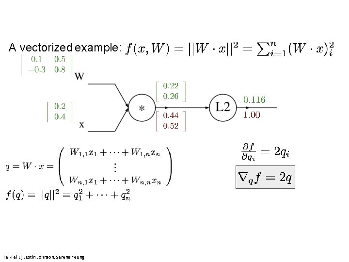
A vectorized example: April 11, 2019 Lecture 4 - 188 Fei-Fei Li, Justin Johnson, Serena Yeung

A vectorized example: April 11, 2019 Lecture 4 - 189 Fei-Fei Li, Justin Johnson, Serena Yeung

A vectorized example: April 11, 2019 Lecture 4 - 190 Fei-Fei Li, Justin Johnson, Serena Yeung

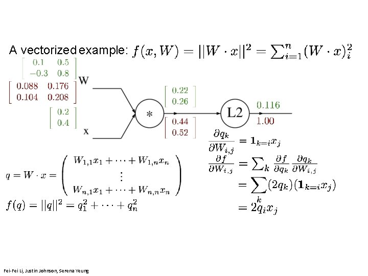
A vectorized example: Lecture 4 - 191 Fei-Fei Li, Justin Johnson, Serena Yeung

A vectorized example: Lecture 4 - 192 Fei-Fei Li, Justin Johnson, Serena Yeung

A vectorized example: April 11, 2019 Lecture 4 - 193 Fei-Fei Li, Justin Johnson, Serena Yeung

A vectorized example: April 11, 2019 Lecture 4 - 194 Fei-Fei Li, Justin Johnson, Serena Yeung

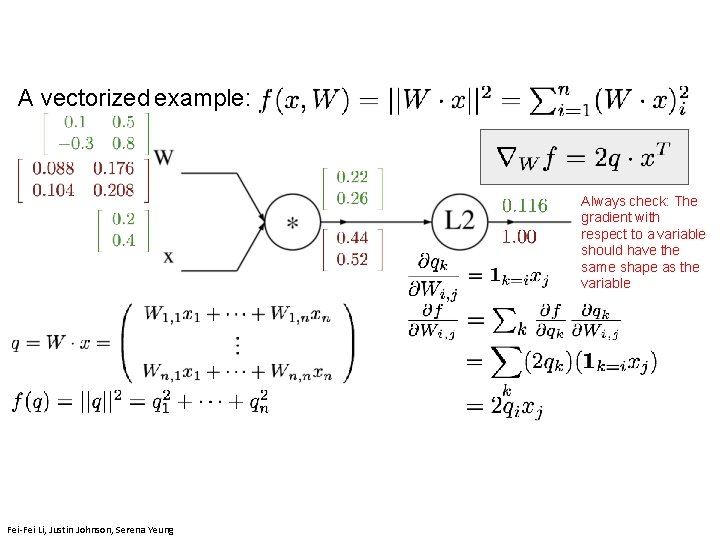
A vectorized example: April 11, 2019 Lecture 4 - 195 Fei-Fei Li, Justin Johnson, Serena Yeung

A vectorized example: Always check: The gradient with respect to a variable should have the same shape as the variable April 11, 2019 Lecture 4 - 196 Fei-Fei Li, Justin Johnson, Serena Yeung