The Limitations of Deep Learning in Adversarial Settings

The Limitations of Deep Learning in Adversarial Settings ECE 693

Deep learning • Large neural networks, recast as deep neural networks (DNNs) in the mid 2000 s, altered the machine learning landscape by outperforming other approaches in many tasks. This was made possible by advances that reduced the computational complexity of training [20]. For instance, Deep learning (DL) can now take advantage of large datasets to achieve accuracy rates higher than previous classification techniques. • This increasing use of deep learning is creating incentives for adversaries to manipulate DNNs to force misclassification of inputs. For instance, applications of deep learning use image classifiers to distinguish inappropriate from appropriate content, and text and image classifiers to differentiate between SPAM and non. SPAM email. An adversary able to craft misclassified inputs would profit from evading detection–indeed such attacks occur today on non-DL classification systems [6], [7], [22]. • In the physical domain, consider a driverless car system that uses DL to identify traffic signs [12]. If slightly altering “STOP” signs causes DNNs to misclassify them, the car would not stop, thus subverting the car’s safety.

adversarial sample • An adversarial sample is an input crafted to cause deep learning algorithms to misclassify. Note that adversarial samples are created at test time, after the DNN has been trained by the defender, and do not require any alteration of the training process. • Figure 1 (next slide) shows examples of adversarial samples taken from our validation experiments. It shows how an image originally showing a digit can be altered to force a DNN to classify it as another digit.

Adversarial sample generation - Distortion is added to input samples to force the DNN to output adversary selected classification (min distortion = 0: 26%, max distortion = 13: 78%, and average distortion " = 4: 06%).

How to create adversarial samples? • Adversarial samples are created from benign samples by adding distortions exploiting the imperfect generalization learned by DNNs from finite training sets [4], and the underlying linearity of most components used to build DNNs [18]. • Previous work explored DNN properties that could be used to craft adversarial samples [18], [30], [36]. • Simply put, these old techniques exploit gradients computed by network training algorithms. In those schemes, instead of using these gradients to update network parameters as would normally be done, gradients are used to update the original input itself, which is subsequently misclassified by DNNs.

This paper: From attacker viewpoint • In this paper, we describe a new class of algorithms for adversarial sample creation against any feedforward (acyclic) DNN [31] and formalize threat model space of deep learning with respect to the integrity of output classification. • Unlike previous approaches mentioned above, we compute a direct mapping from the input to the output to achieve an explicit adversarial goal. • Furthermore, our approach only alters a (frequently small) fraction of input features leading to reduced perturbation of the source inputs. It also enables adversaries to apply heuristic searches to find perturbations leading to input targeted misclassifications (perturbing inputs to result in a specific output classification).

Problem modeling • More formally, a DNN models a multidimensional function F : X Y where X is a (raw) feature vector and Y is an output vector. We construct an adversarial sample X from a benign sample X by adding a perturbation vector X by solving the following optimization problem: Is the adversarial sample.

Solve such an attack Model • Y is the desired adversarial output, and ||. || is a norm appropriate to compare the DNN inputs. Solving this problem is non-trivial, as properties of DNNs make it non-linear and non-convex [25]. • Thus, we craft adversarial samples by constructing a mapping from input perturbations to output variations. Note that all research mentioned above took the opposite approach: it used output variations to find corresponding input perturbations. • Our understanding of how changes made to inputs affect a DNN’s output stems from the evaluation of the forward derivative: a matrix we introduce and define as the Jacobian of the function learned by the DNN. • The forward derivative is used to construct adversarial saliency maps indicating input features to include in perturbation X in order to produce adversarial samples inducing a certain behavior from the DNN.

Model • Forward derivatives approaches are much more powerful than gradient descent techniques used in prior systems. They are applicable to both supervised and unsupervised architectures and allow adversaries to generate information for broad families of adversarial samples. • Indeed, adversarial saliency maps are versatile tools based on the forward derivative and designed with adversarial goals in mind, giving greater control to adversaries with respect to the choice of perturbations. • In our work, we consider the following questions to formalize the security of DL in adversarial settings: (1) “What is the minimal knowledge required to perform attacks against DL? ”, (2) “How can vulnerable or resistant samples be identified? ”, and (3) “How are adversarial samples perceived by humans? ”.

Paper contributions • We formalize the space of adversaries against classification DNNs with respect to adversarial goal and capabilities (i. e. , from attacker’s perspective). Here, we provide a better understanding of how attacker capabilities constrain attack strategies and goals. • We introduce a new class of algorithms for crafting adversarial samples solely by using knowledge of the DNN architecture. These algorithms (1) exploit forward derivatives that inform the learned behavior of DNNs, and (2) build adversarial saliency maps enabling an efficient exploration of the adversarial-samples search space. • We validate the algorithms using a widely used computer vision DNN. We define and measure sample distortion and source-to-target hardness, and explore defenses against adversarial samples. We conclude by studying human perception of distorted samples.

Taxonomy • Threat Model Taxonomy: our class of algorithms operates in the threat model indicated by a star. Here an attacker knows everything; thus can attack the system more easily.

Adversarial Goals • Threats are defined with a specific function to be protected/defended. In the case of deep learning systems, the integrity of the classification is of paramount importance. Specifically, an adversary of a deep learning system seeks to provide an input X that results in an incorrect output classification. 1) Confidence reduction - reduce the output classification confidence level (thereby introducing class ambiguity) -- just want to make system less reliable. 2) Misclassification - alter the output classification to any class different from the original class 3) Targeted misclassification - produce inputs (any inputs) that force the output classification to be a specific target class. 4) Source/target misclassification - force the output classification of a specific input to be a specific target class.

Strongest attacker • Training data and network architecture - This adversary has perfect knowledge of the neural network used for classification. The attacker has to access the training data T, functions and algorithms used for network training, and is able to extract knowledge about the DNN’s architecture F. • This includes the number and type of layers, the activation functions of neurons, as well as weight and bias matrices. He also knows which algorithm was used to train the network, including the associated loss function c. This is the strongest adversary that can analyze the training data and simulate the deep neural network.

Second strongest attacker • Network architecture - This adversary has knowledge of the network architecture F and its parameter values. For instance, this corresponds to an adversary who can collect information about both (1) the layers and activation functions used to design the neural network, and (2) the weights and biases resulting from the training phase. This gives the adversary enough information to simulate the network. Our algorithms assume this threat model, and show a new class of algorithms that generate adversarial samples for supervised and unsupervised feedforward DNNs.

Third strongest attacker • Training data - This adversary is able to collect a surrogate dataset, sampled from the same distribution that the original dataset used to train the DNN. However, the attacker is not aware of the architecture used to design the neural network. • Thus, typical attacks conducted in this model would likely include training commonly deployed deep learning architectures using the surrogate dataset to approximate the model learned by the legitimate classifier.

Weaker attackers • Oracle - This adversary has the ability to use the neural network (or a proxy of it) as an “oracle”. Here the adversary can obtain output classifications from supplied inputs (much like a chosen-plaintext attack in cryptography). This enables differential attacks, where the adversary can observe the relationship between changes in inputs and outputs (continuing with the analogy, such as used in differential cryptanalysis) to adaptively craft adversarial samples. This adversary can be further parameterized by the number of absolute or rate-limited input/output trials they may perform. • Samples only - This adversary has the ability to collect pairs of input and output related to the neural network classifier. However, he cannot modify these inputs to observe the difference in the output. (To continue the cryptanalysis analogy, this threat model would correspond to a known plaintext attack. ) These pairs are largely labeled output data, and intuition states that they would most likely only be useful in very large quantities.

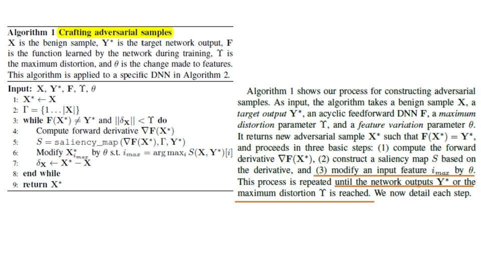
Algorithm’s design goal • In this section, we present a general algorithm for modifying samples so that a DNN yields any adversarial output. • We later validate this algorithm by having a classifier misclassify samples into a chosen target class. • This algorithm captures adversaries crafting samples in the setting corresponding to the upper right-hand corner of Figure 2. We show that knowledge of the architecture and weight parameters are sufficient to derive adversarial samples against acyclic feedforward DNNs. • This requires evaluating the DNN’s forward derivative in order to construct an adversarial saliency map that identifies the set of input features relevant to the adversary’s goal. • Perturbing the features identified in this way quickly leads to the desired adversarial output, for instance misclassification. Although we describe our approach with supervised neural networks used as classifiers, it also applies to unsupervised architectures.

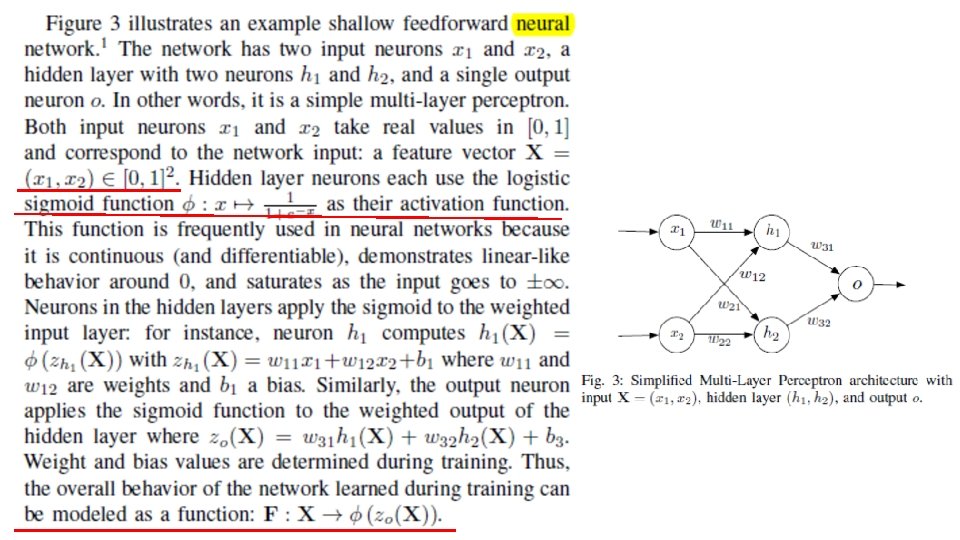
On DNN • Deep neural networks (DNNs) are large neural networks organized into layers of neurons, corresponding to successive representations of the input data. A neuron is an individual computing unit transmitting to other neurons the result of the application of its activation function on its input. • Neurons are connected by links with different weights and biases characterizing the strength between neuron pairs. • Weights and biases can be viewed as DNN parameters used for information storage. We define a network architecture to include knowledge of the network topology, neuron activation functions, as well as weight and bias values. • Weights and biases are determined during training by finding values that minimize a cost function c evaluated over the training data T. Network training is traditionally done by gradient descent using backpropagation.

supervised or unsupervised • Deep learning can be partitioned in two categories, depending on whether DNNs are trained in a supervised or unsupervised manner [29]. • Supervised training leads to models that map unseen samples using a function inferred from labeled training data. • On the contrary, unsupervised training learns representations of unlabeled training data, and resulting DNNs can be used to generate new samples, or to automate feature engineering by acting as a pre-processing layer for larger DNNs. • We restrict ourselves to the problem of learning multi-classifiers in supervised settings. These DNNs are given an input X and output a class probability vector Y. • Note that our work here remains valid for unsupervised-trained DNNs, .

• Fig. 3 example’s low dimensionality allows us to better understand the underlying concepts behind our algorithms. We indeed show small input perturbations found using the forward derivative can induce large variations of the neural network output. Assuming that input biases b 1, b 2, and b 3 are null, we train this toy network to learn the

• We are now going to demonstrate how to craft adversarial samples on this neural network. The adversary considers a legitimate sample X, classified as F(X) = Y by the network, compare points in the input domain. Informally, the adversary is searching for small perturbations of the input that will incur a modification of the output into Y. Finding these perturbations can be done using optimization techniques, simple heuristics, or even brute force. However such solutions are hard to implement for deep neural networks because of non-convexity and non-linearity [25]. Instead, we propose a systematic approach stemming from the forward derivative.

Forward Derivative • We define the forward derivative as the Jacobian matrix of the function F learned by the neural network during training. • For this example, the output of F is one dimensional, the matrix is therefore reduced to a vector:

forward derivative result • The forward derivative for our example network is illustrated in Figure 5

forward derivative can visualize the boundary • This plot (Fig. 5) makes it easy to visualize the divide between the network’s two possible outputs in terms of values assigned to the input feature x 2: 0 to the left of the spike, and 1 to its left. • Notice that this aligns with Figure 4, and gives us the information needed to achieve our adversarial goal: find input perturbations that drive the output closer to a desired value.

• Consulting Figure 5 alongside our example network, we can confirm this intuition by looking at a few sample points. Consider X = (1, 0. 37) and X = (1, 0. 43), which are both located near the spike in Figure 5. Although they only differ by a small amount (Δx = 0. 05), they cause a significant change in the network’s output, as F(X) = 0. 11 and F(X) = 0. 95.

forward derivative tells us a lot … • the forward derivative tells us which input regions are unlikely to yield adversarial samples, and are thus more immune to adversarial manipulations. Notice in Figure 5 that when either input (x 1, X 2) is close to 0, the forward derivative is small. This aligns with our intuition that it will be more difficult to find adversarial samples close to (1, 0) than (1, 0. 4). • This tells the adversary to focus on features corresponding to larger forward derivative values in a given input when constructing a sample, making his search more efficient and ultimately leading to smaller overall distortions. • The takeaways of this example are thereby: (1) small input variations can lead to extreme variations of the output of the neural network, (2) not all regions from the input domain are conducive to find adversarial samples, and (3) the forward derivative reduces the adversarial-sample search space (i. e. , makes it easier to generate an input attack).

forward derivative : Generalizing to Feedforward Deep Neural Networks

How to Solve forward derivative : For K-th hidden layer: Because H(. ) is X’s function, we have: For final output layer:

Adversarial Saliency Maps • We extend saliency maps previously introduced as visualization tools [34] to construct adversarial saliency maps. These maps indicate which input features an adversary should perturb in order to affect the desired changes in network output most efficiently, and are thus versatile tools that allow adversaries to generate broad classes of adversarial samples. • Adversarial saliency maps are defined to suit problem specific adversarial goals. For instance, we later study a network used as a classifier, its output is a probability vector (i. e. , multiple probability values) across classes, where the final predicted class value corresponds to the component with the highest probability:

Definition of saliency map • In our case, the saliency map is therefore based on the forward derivative, as this gives the adversary the information needed to cause the neural network to misclassify a given sample. More precisely, the adversary wants to misclassify a sample Here: X – input features; t, j ---- output class F --- DL function əF/əx – Forward derivative

Find the proper “input features” which causes increasing “saliency” prob if we target a specific “output class”.

i. e. , input features!

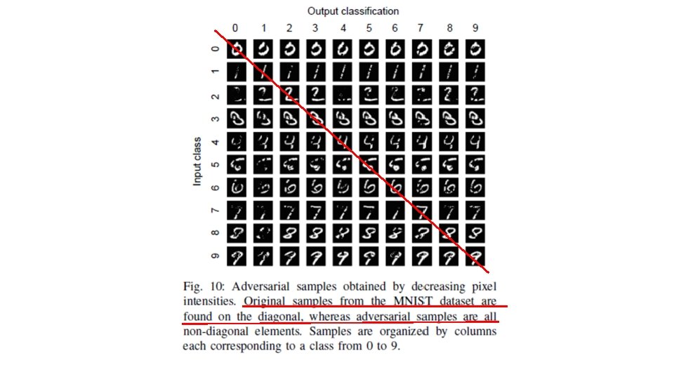
APPLICATION OF THE APPROACH • In the above we have formally described a class of algorithms for crafting adversarial samples misclassified by feedforward DNNs using three tools: the forward derivative, adversarial saliency maps, and the crafting algorithm. • We now apply these tools to a DNN used for a computer vision classification task: handwritten digit recognition. We show that our algorithms successfully craft adversarial samples from any source class to any given target class, which for this application means that any digit can be perturbed so that it is misclassified as any other digit.

Saliency map: subroutine saliency_map generates a map defining which input features (here we assume 2 features) will be modified at each iteration.

Input attack • Adversarial samples generated by feeding the crafting algorithm an empty input. Each sample produced corresponds to one target class from 0 to 9. Interestingly, for classes 0, 2, 3 and 5, humans can clearly recognize the target digit.