CS 7643 Deep Learning Topics Stride padding Pooling

CS 7643: Deep Learning Topics: – – Stride, padding Pooling layers Fully-connected layers as convolutions Backprop in conv layers Dhruv Batra Georgia Tech

Invited Talks • Sumit Chopra on CNNs for Pixel Labeling – Head of AI Research @ Imagen Technologies • Previously Facebook AI Research – Tue 09/26, in class (C) Dhruv Batra 2

Administrativia • HW 1 due soon – 09/22 • HW 2 + PS 2 both coming out on 09/22 • Note on class schedule coming up – Switching to paper reading starting next week. – https: //docs. google. com/spreadsheets/d/1 u. N 31 Yc. WAG 6 nhjv YPUVKMy 3 v. Hw. W-h 9 MZCe 8 y. KCqw 0 Rs. U/edit#gid=0 • First review due: Tue 09/26 • First student presentation due: Thr 09/28 (C) Dhruv Batra 3

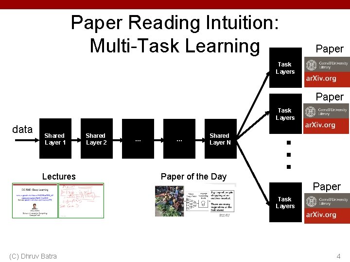
Paper Reading Intuition: Multi-Task Learning Task Layers data Shared Layer 1 Lectures Shared Layer 2 … … Shared Layer N Paper of the Day Task Layers (C) Dhruv Batra Paper 2 . . . Task Layers Paper 1 Paper 6 4

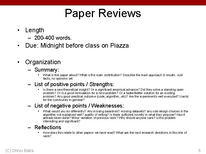
Paper Reviews • Length – 200 -400 words. • Due: Midnight before class on Piazza • Organization – Summary: • What is this paper about? What is the main contribution? Describe the main approach & results. Just facts, no opinions yet. – List of positive points / Strengths: • Is there a new theoretical insight? Or a significant empirical advance? Did they solve a standing open problem? Or is a good formulation for a new problem? Or a faster/better solution for an existing problem? Any good practical outcome (code, algorithm, etc)? Are the experiments well executed? Useful for the community in general? – List of negative points / Weaknesses: • What would you do differently? Any missing baselines? missing datasets? any odd design choices in the algorithm not explained well? quality of writing? Is there sufficient novelty in what they propose? Has it already been done? Minor variation of previous work? Why should anyone care? Is the problem interesting and significant? – Reflections • (C) Dhruv Batra How does this relate to other papers we have read? What are the next research directions in this line of work? 5

Presentations • Frequency – Once in the semester: 5 min presentation. • Expectations – Present details of 1 paper • Describe formulation, experiment, approaches, datasets • Encouraged to present a broad picture • Show results, videos, gifs, etc. – Please clearly cite the source of each slide that is not your own. – Meet with TA 1 week before class to dry run presentation • Worth 40% of presentation grade (C) Dhruv Batra 6

Administrativia • Project Teams Google Doc – https: //docs. google. com/spreadsheets/d/1 Aa. XY 0 JE 4 l. Ab. Hvo Da. Wlc 9 zsmf. KMyu. GS 39 JAn 9 dpe. Xhh. Q/edit#gid=0 – Project Title – 1 -3 sentence project summary TL; DR – Team member names + GT IDs (C) Dhruv Batra 7

Recap of last time (C) Dhruv Batra 8

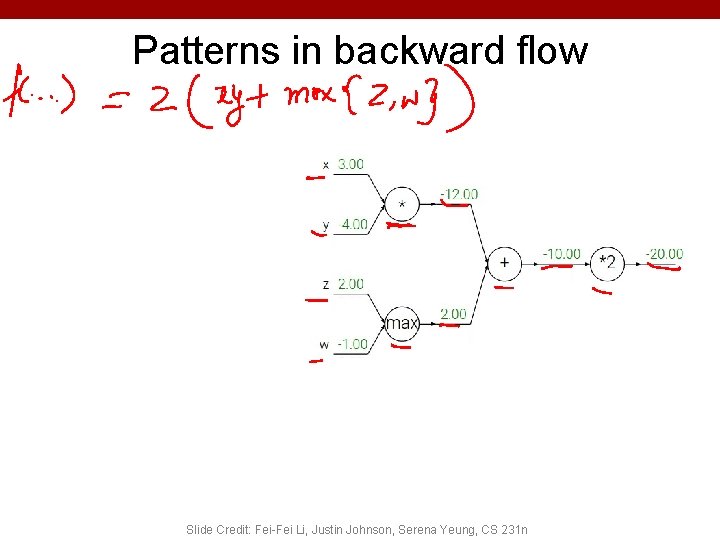
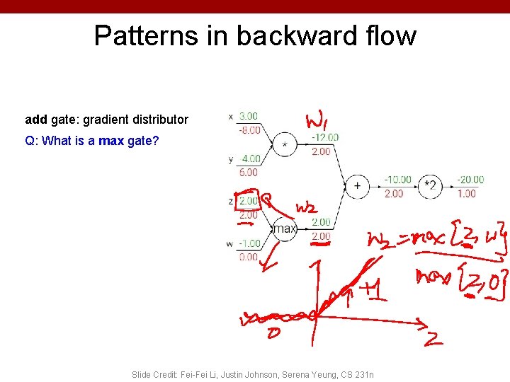
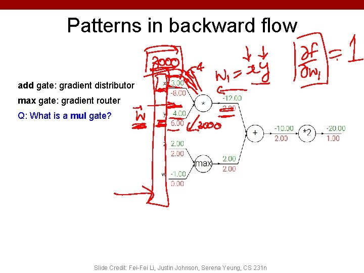
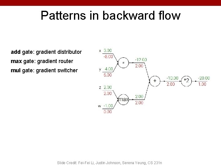
Patterns in backward flow Slide Credit: Fei-Fei Li, Justin Johnson, Serena Yeung, CS 231 n

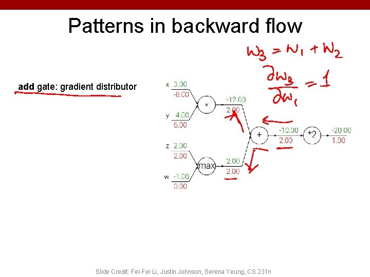
Patterns in backward flow add gate: gradient distributor Slide Credit: Fei-Fei Li, Justin Johnson, Serena Yeung, CS 231 n

Patterns in backward flow add gate: gradient distributor Q: What is a max gate? Slide Credit: Fei-Fei Li, Justin Johnson, Serena Yeung, CS 231 n

Patterns in backward flow add gate: gradient distributor max gate: gradient router Q: What is a mul gate? Slide Credit: Fei-Fei Li, Justin Johnson, Serena Yeung, CS 231 n

Patterns in backward flow add gate: gradient distributor max gate: gradient router mul gate: gradient switcher Slide Credit: Fei-Fei Li, Justin Johnson, Serena Yeung, CS 231 n

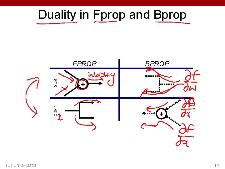
Duality in Fprop and Bprop COPY SUM FPROP (C) Dhruv Batra BPROP + + 14

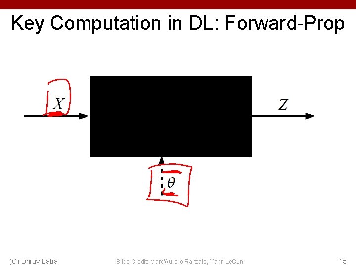
Key Computation in DL: Forward-Prop (C) Dhruv Batra Slide Credit: Marc'Aurelio Ranzato, Yann Le. Cun 15

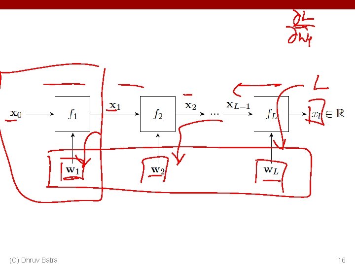
(C) Dhruv Batra 16

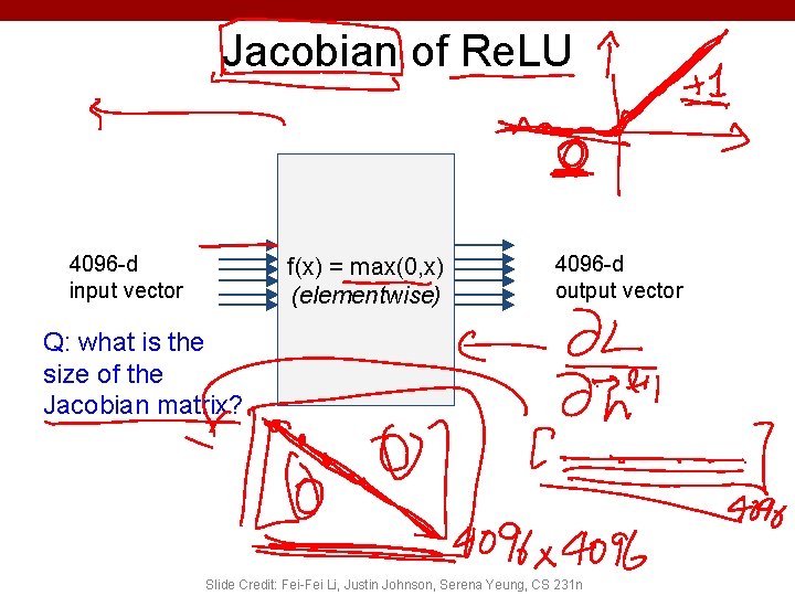
Jacobian of Re. LU 4096 -d input vector f(x) = max(0, x) (elementwise) 4096 -d output vector Q: what is the size of the Jacobian matrix? 17 Slide Credit: Fei-Fei Li, Justin Johnson, Serena Yeung, CS 231 n

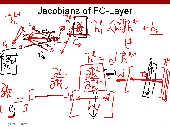
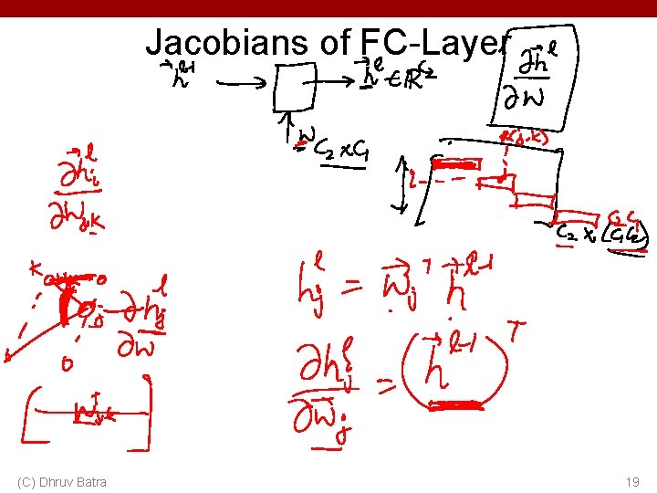
Jacobians of FC-Layer (C) Dhruv Batra 18

Jacobians of FC-Layer (C) Dhruv Batra 19

Convolutional Neural Networks (without the brain stuff) Slide Credit: Fei-Fei Li, Justin Johnson, Serena Yeung, CS 231 n

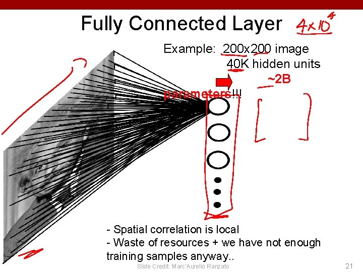
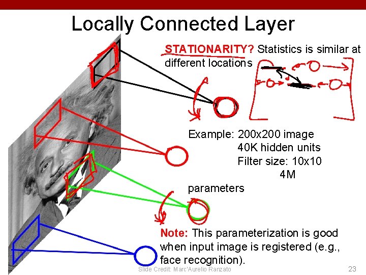
Fully Connected Layer Example: 200 x 200 image 40 K hidden units ~2 B parameters!!! - Spatial correlation is local - Waste of resources + we have not enough training samples anyway. . Slide Credit: Marc'Aurelio Ranzato 21

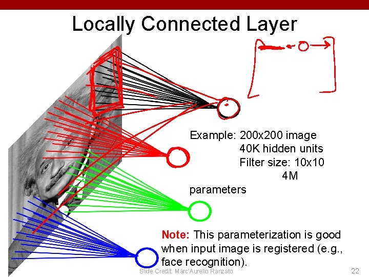
Locally Connected Layer Example: 200 x 200 image 40 K hidden units Filter size: 10 x 10 4 M parameters Note: This parameterization is good when input image is registered (e. g. , face recognition). Slide Credit: Marc'Aurelio Ranzato 22

Locally Connected Layer STATIONARITY? Statistics is similar at different locations Example: 200 x 200 image 40 K hidden units Filter size: 10 x 10 4 M parameters Note: This parameterization is good when input image is registered (e. g. , face recognition). Slide Credit: Marc'Aurelio Ranzato 23

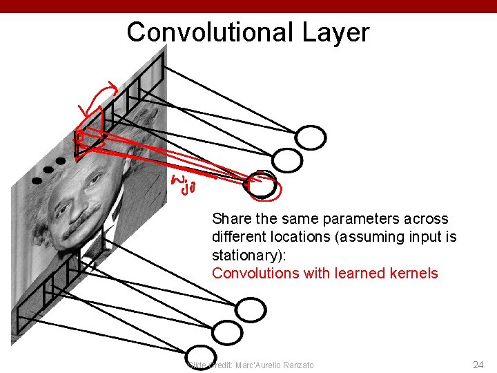
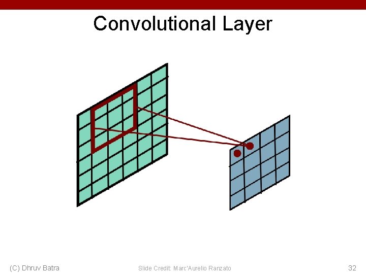
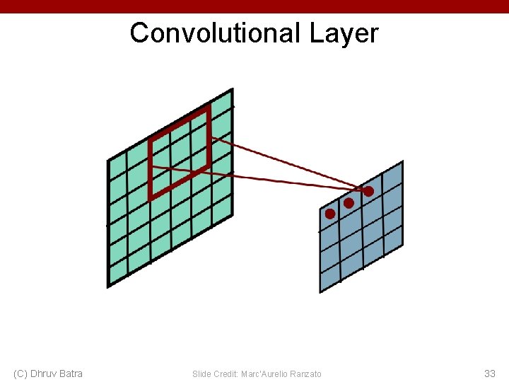
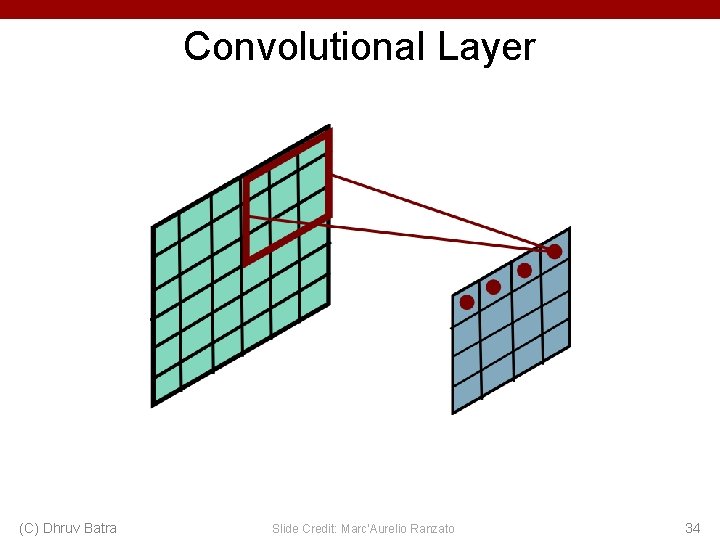
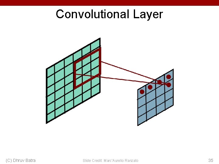
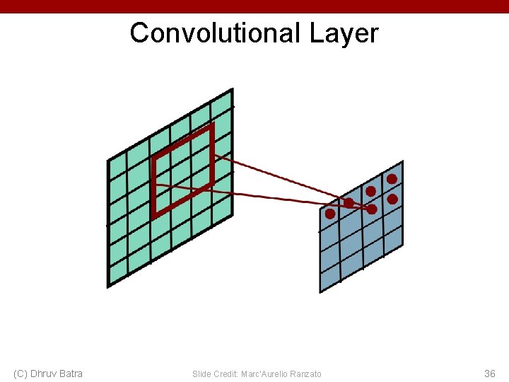
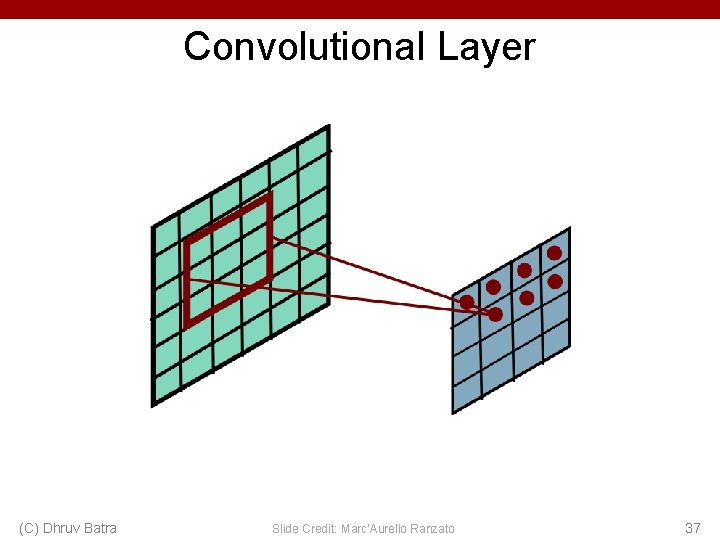
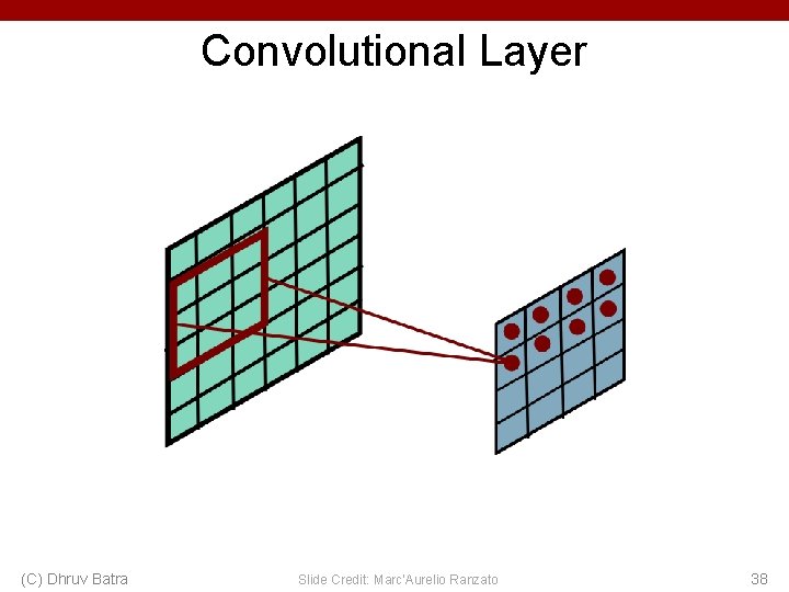
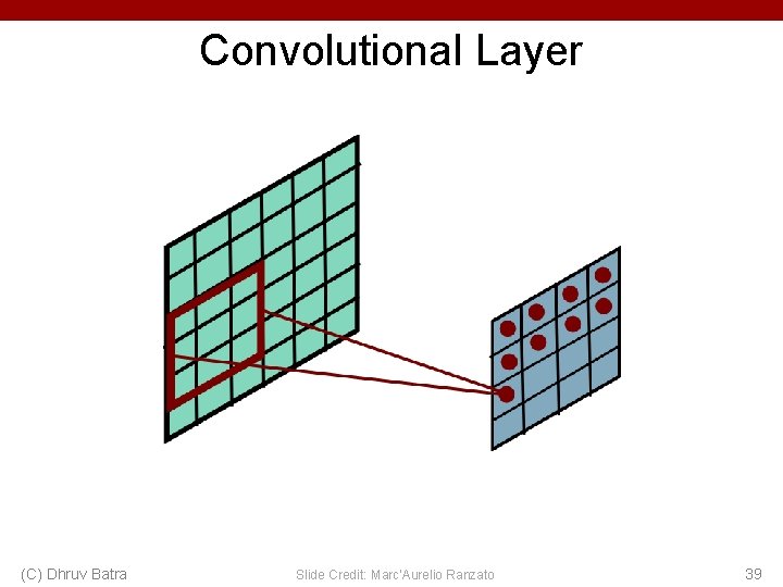
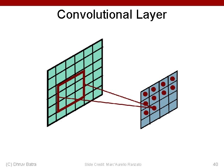
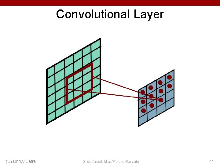
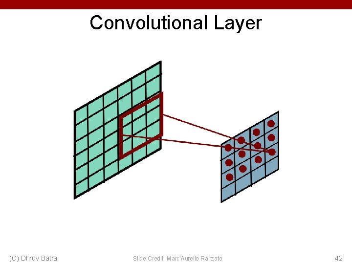
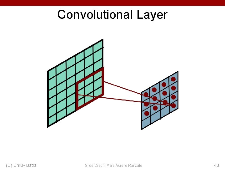
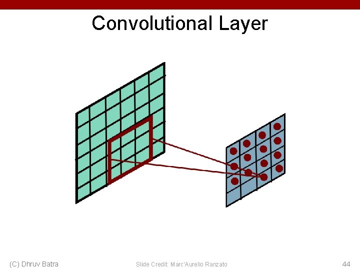
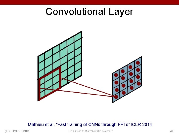
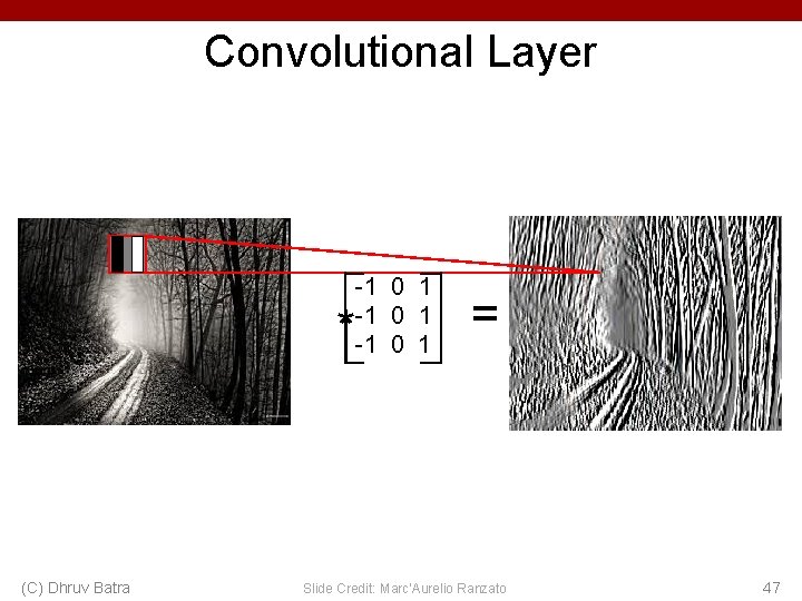
Convolutional Layer Share the same parameters across different locations (assuming input is stationary): Convolutions with learned kernels Slide Credit: Marc'Aurelio Ranzato 24

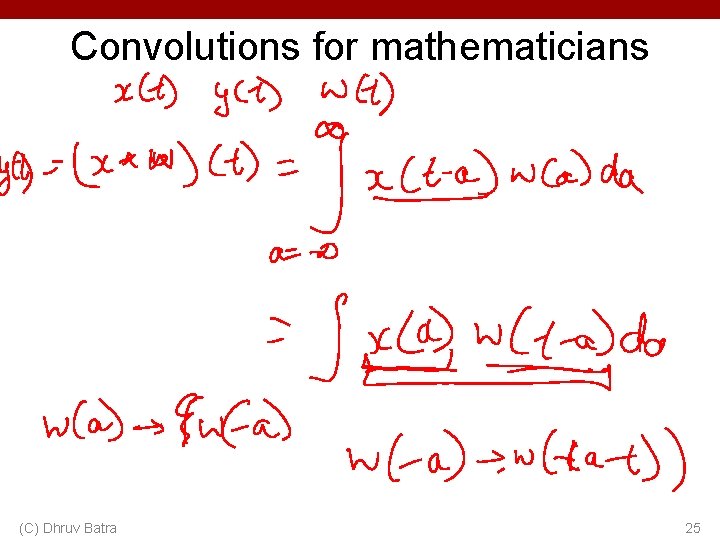
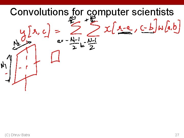
Convolutions for mathematicians (C) Dhruv Batra 25

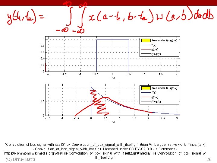
"Convolution of box signal with itself 2" by Convolution_of_box_signal_with_itself. gif: Brian Ambergderivative work: Tinos (talk) - Convolution_of_box_signal_with_itself. gif. Licensed under CC BY-SA 3. 0 via Commons https: //commons. wikimedia. org/wiki/File: Convolution_of_box_signal_with_itself 2. gif#/media/File: Convolution_of_box_signal_wi th_itself 2. gif (C) Dhruv Batra 26

Convolutions for computer scientists (C) Dhruv Batra 27

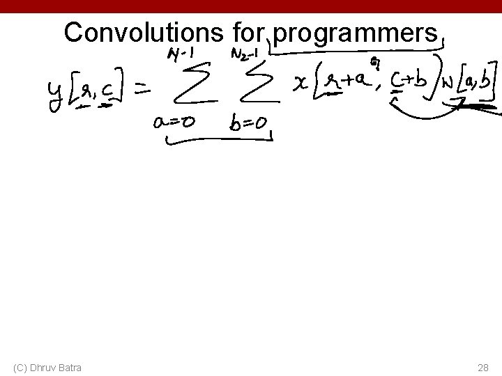
Convolutions for programmers (C) Dhruv Batra 28

Convolution Explained • http: //setosa. io/ev/image-kernels/ • https: //github. com/bruckner/deep. Viz (C) Dhruv Batra 29

Plan for Today • Convolutional Neural Networks – – (C) Dhruv Batra Stride, padding Pooling layers Fully-connected layers as convolutions Backprop in conv layers 30

Convolutional Layer (C) Dhruv Batra Slide Credit: Marc'Aurelio Ranzato 31

Convolutional Layer (C) Dhruv Batra Slide Credit: Marc'Aurelio Ranzato 32

Convolutional Layer (C) Dhruv Batra Slide Credit: Marc'Aurelio Ranzato 33

Convolutional Layer (C) Dhruv Batra Slide Credit: Marc'Aurelio Ranzato 34

Convolutional Layer (C) Dhruv Batra Slide Credit: Marc'Aurelio Ranzato 35

Convolutional Layer (C) Dhruv Batra Slide Credit: Marc'Aurelio Ranzato 36

Convolutional Layer (C) Dhruv Batra Slide Credit: Marc'Aurelio Ranzato 37

Convolutional Layer (C) Dhruv Batra Slide Credit: Marc'Aurelio Ranzato 38

Convolutional Layer (C) Dhruv Batra Slide Credit: Marc'Aurelio Ranzato 39

Convolutional Layer (C) Dhruv Batra Slide Credit: Marc'Aurelio Ranzato 40

Convolutional Layer (C) Dhruv Batra Slide Credit: Marc'Aurelio Ranzato 41

Convolutional Layer (C) Dhruv Batra Slide Credit: Marc'Aurelio Ranzato 42

Convolutional Layer (C) Dhruv Batra Slide Credit: Marc'Aurelio Ranzato 43

Convolutional Layer (C) Dhruv Batra Slide Credit: Marc'Aurelio Ranzato 44

Convolutional Layer (C) Dhruv Batra Slide Credit: Marc'Aurelio Ranzato 45

Convolutional Layer Mathieu et al. “Fast training of CNNs through FFTs” ICLR 2014 (C) Dhruv Batra Slide Credit: Marc'Aurelio Ranzato 46

Convolutional Layer * (C) Dhruv Batra -1 0 1 = Slide Credit: Marc'Aurelio Ranzato 47

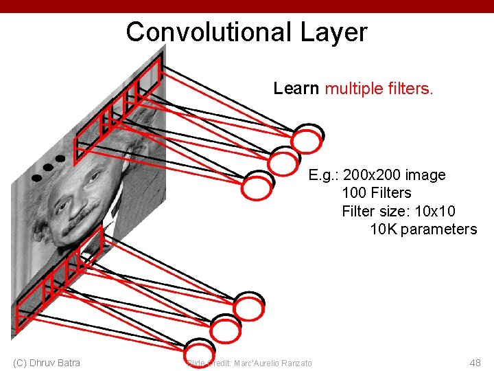
Convolutional Layer Learn multiple filters. E. g. : 200 x 200 image 100 Filters Filter size: 10 x 10 10 K parameters (C) Dhruv Batra Slide Credit: Marc'Aurelio Ranzato 48

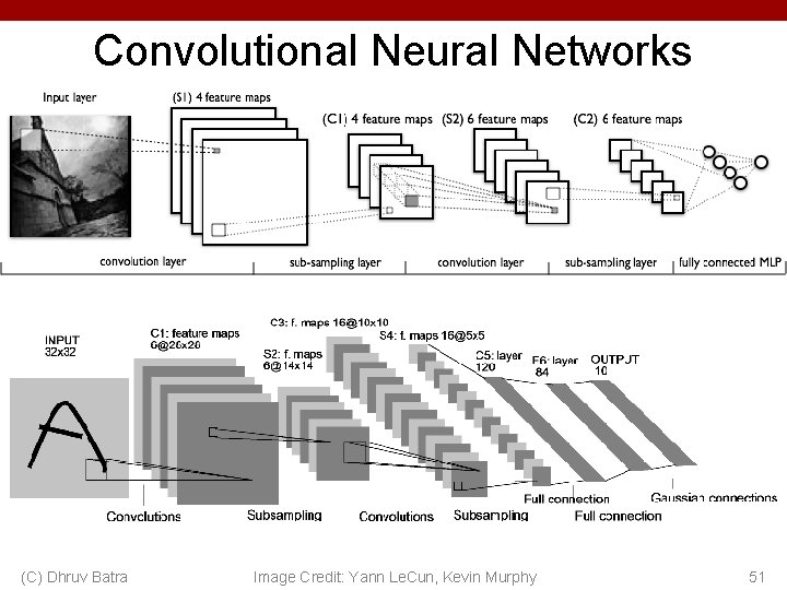
Convolutional Neural Networks a (C) Dhruv Batra Image Credit: Yann Le. Cun, Kevin Murphy 51

FC vs Conv Layer 52

FC vs Conv Layer 53

FC vs Conv Layer 54

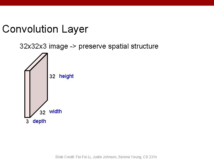
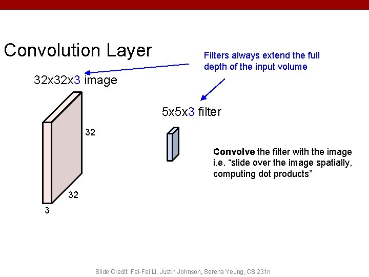
Convolution Layer 32 x 3 image -> preserve spatial structure 32 height 32 width 3 depth Slide Credit: Fei-Fei Li, Justin Johnson, Serena Yeung, CS 231 n

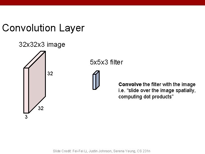
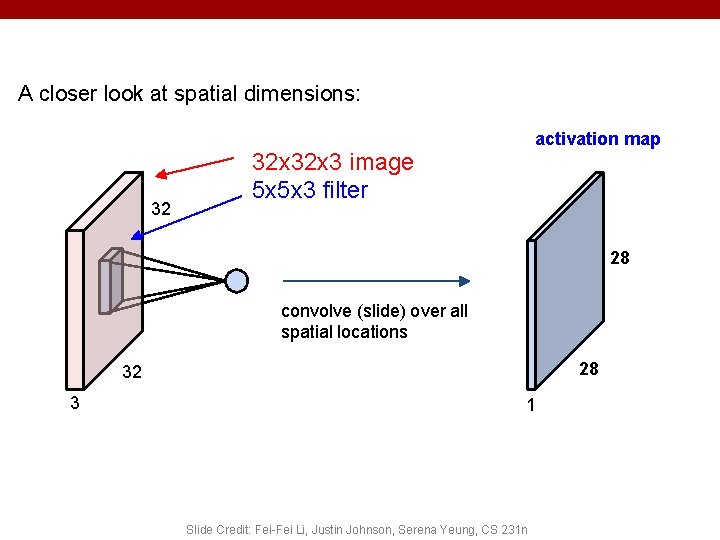
Convolution Layer 32 x 3 image 5 x 5 x 3 filter 32 Convolve the filter with the image i. e. “slide over the image spatially, computing dot products” 32 3 Slide Credit: Fei-Fei Li, Justin Johnson, Serena Yeung, CS 231 n

Convolution Layer Filters always extend the full depth of the input volume 32 x 3 image 5 x 5 x 3 filter 32 Convolve the filter with the image i. e. “slide over the image spatially, computing dot products” 32 3 Slide Credit: Fei-Fei Li, Justin Johnson, Serena Yeung, CS 231 n

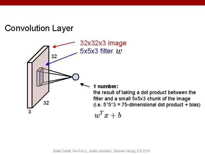
Convolution Layer 32 32 32 x 3 image 5 x 5 x 3 filter 1 number: the result of taking a dot product between the filter and a small 5 x 5 x 3 chunk of the image (i. e. 5*5*3 = 75 -dimensional dot product + bias) 3 Slide Credit: Fei-Fei Li, Justin Johnson, Serena Yeung, CS 231 n

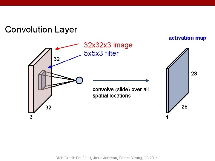
Convolution Layer 32 32 x 3 image 5 x 5 x 3 filter activation map 28 convolve (slide) over all spatial locations 28 32 3 1 Slide Credit: Fei-Fei Li, Justin Johnson, Serena Yeung, CS 231 n

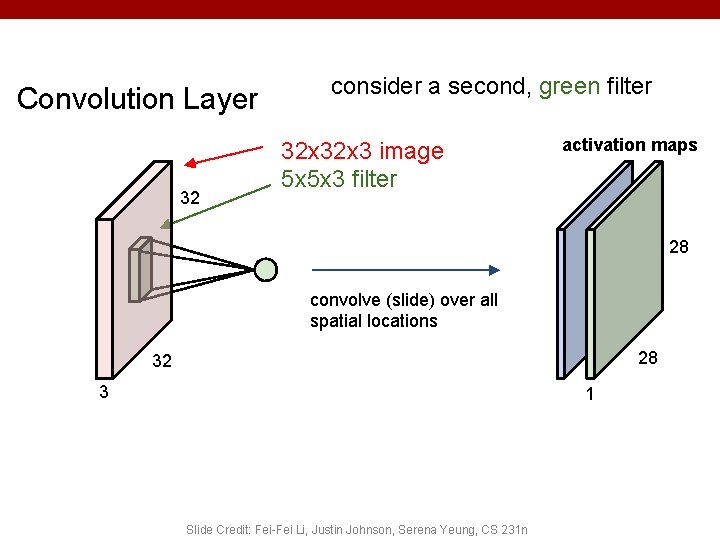
Convolution Layer 32 consider a second, green filter 32 x 3 image 5 x 5 x 3 filter activation maps 28 convolve (slide) over all spatial locations 28 32 3 1 Slide Credit: Fei-Fei Li, Justin Johnson, Serena Yeung, CS 231 n

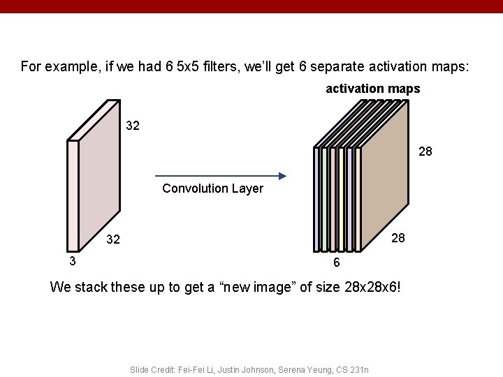
For example, if we had 6 5 x 5 filters, we’ll get 6 separate activation maps: activation maps 32 28 Convolution Layer 28 32 3 6 We stack these up to get a “new image” of size 28 x 6! Slide Credit: Fei-Fei Li, Justin Johnson, Serena Yeung, CS 231 n

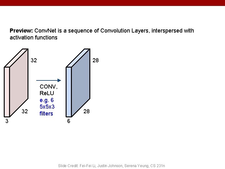
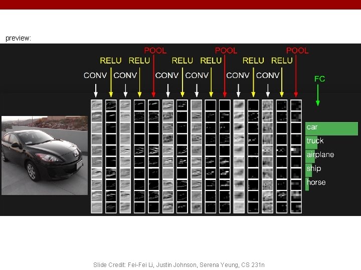
Preview: Conv. Net is a sequence of Convolution Layers, interspersed with activation functions 32 32 3 28 CONV, Re. LU e. g. 6 5 x 5 x 3 filters 28 6 Slide Credit: Fei-Fei Li, Justin Johnson, Serena Yeung, CS 231 n

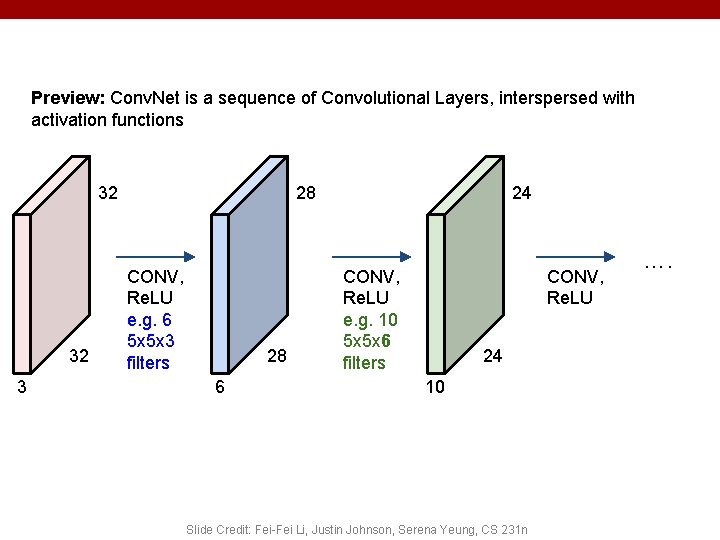
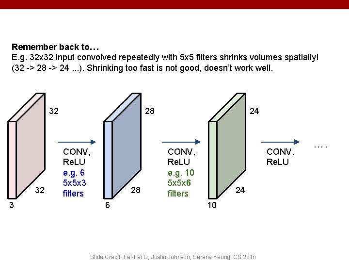
Preview: Conv. Net is a sequence of Convolutional Layers, interspersed with activation functions 32 32 3 28 CONV, Re. LU e. g. 6 5 x 5 x 3 filters 28 6 24 CONV, Re. LU e. g. 10 5 x 5 x 6 filters CONV, Re. LU 24 10 Slide Credit: Fei-Fei Li, Justin Johnson, Serena Yeung, CS 231 n ….

Preview [Zeiler and Fergus 2013] Slide Credit: Fei-Fei Li, Justin Johnson, Serena Yeung, CS 231 n Visualization of VGG-16 by Lane Mc. Intosh. VGG-16 architecture from [Simonyan and Zisserman 2014].

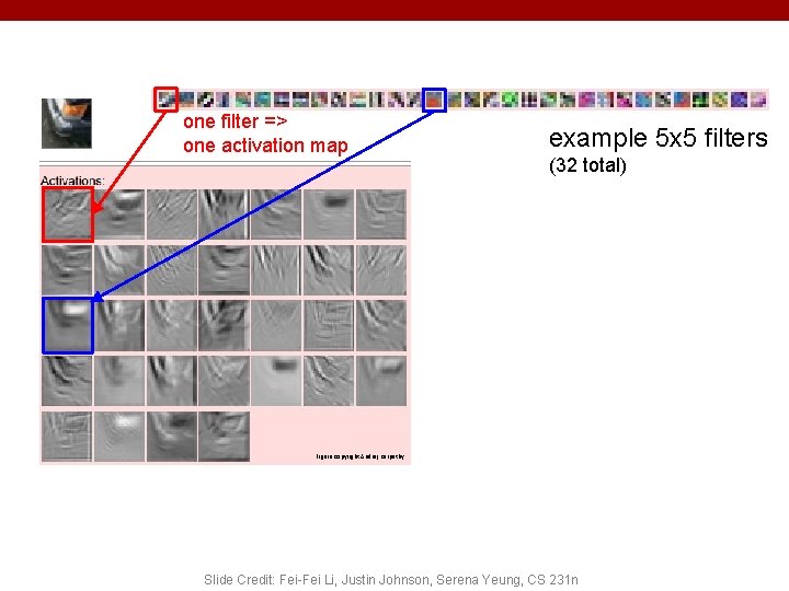
one filter => one activation map example 5 x 5 filters (32 total) Figure copyright Andrej Karpathy. Slide Credit: Fei-Fei Li, Justin Johnson, Serena Yeung, CS 231 n

Convolutional Neural Networks a (C) Dhruv Batra Image Credit: Yann Le. Cun, Kevin Murphy 66

preview: Slide Credit: Fei-Fei Li, Justin Johnson, Serena Yeung, CS 231 n

A closer look at spatial dimensions: 32 activation map 32 x 3 image 5 x 5 x 3 filter 28 convolve (slide) over all spatial locations 28 32 3 1 Slide Credit: Fei-Fei Li, Justin Johnson, Serena Yeung, CS 231 n

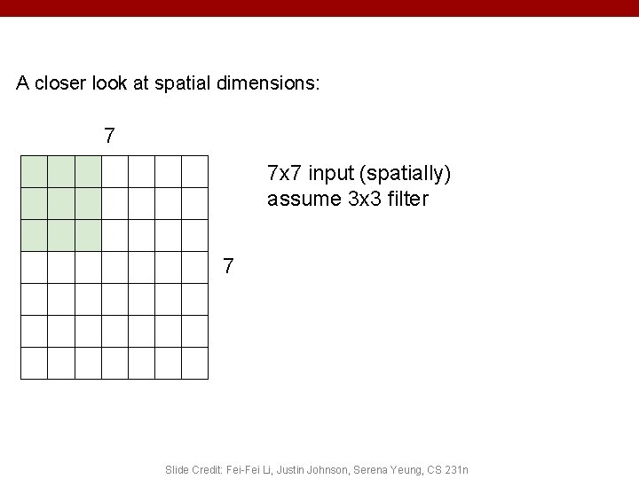
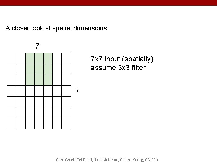
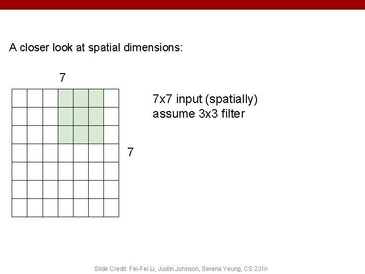
A closer look at spatial dimensions: 7 7 x 7 input (spatially) assume 3 x 3 filter 7 Slide Credit: Fei-Fei Li, Justin Johnson, Serena Yeung, CS 231 n

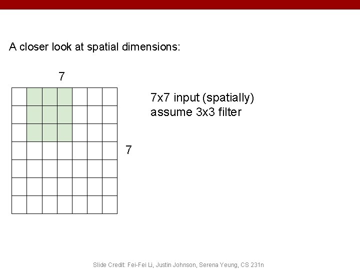
A closer look at spatial dimensions: 7 7 x 7 input (spatially) assume 3 x 3 filter 7 Slide Credit: Fei-Fei Li, Justin Johnson, Serena Yeung, CS 231 n

A closer look at spatial dimensions: 7 7 x 7 input (spatially) assume 3 x 3 filter 7 Slide Credit: Fei-Fei Li, Justin Johnson, Serena Yeung, CS 231 n

A closer look at spatial dimensions: 7 7 x 7 input (spatially) assume 3 x 3 filter 7 Slide Credit: Fei-Fei Li, Justin Johnson, Serena Yeung, CS 231 n

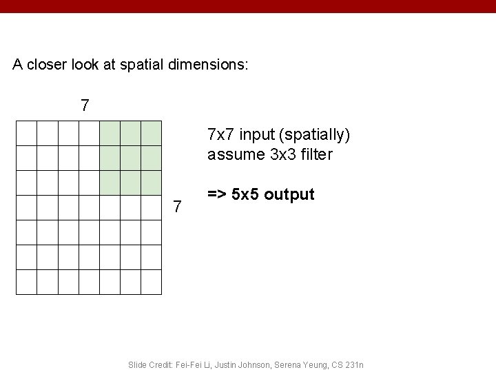
A closer look at spatial dimensions: 7 7 x 7 input (spatially) assume 3 x 3 filter 7 => 5 x 5 output Slide Credit: Fei-Fei Li, Justin Johnson, Serena Yeung, CS 231 n

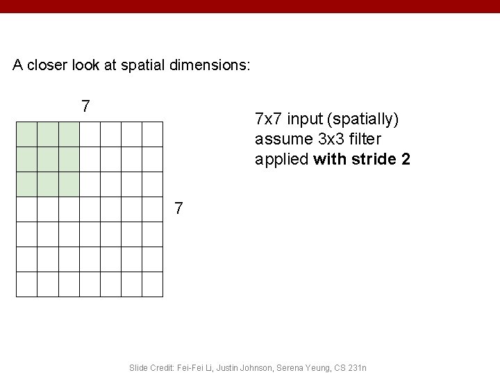
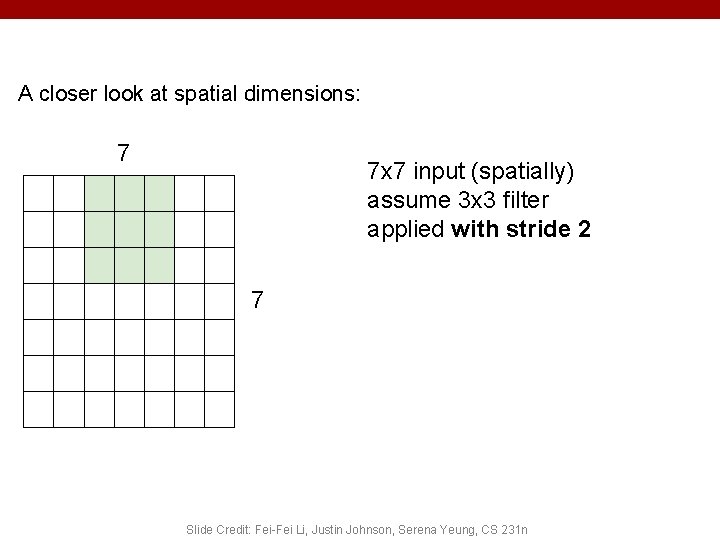
A closer look at spatial dimensions: 7 7 x 7 input (spatially) assume 3 x 3 filter applied with stride 2 7 Slide Credit: Fei-Fei Li, Justin Johnson, Serena Yeung, CS 231 n

A closer look at spatial dimensions: 7 7 x 7 input (spatially) assume 3 x 3 filter applied with stride 2 7 Slide Credit: Fei-Fei Li, Justin Johnson, Serena Yeung, CS 231 n

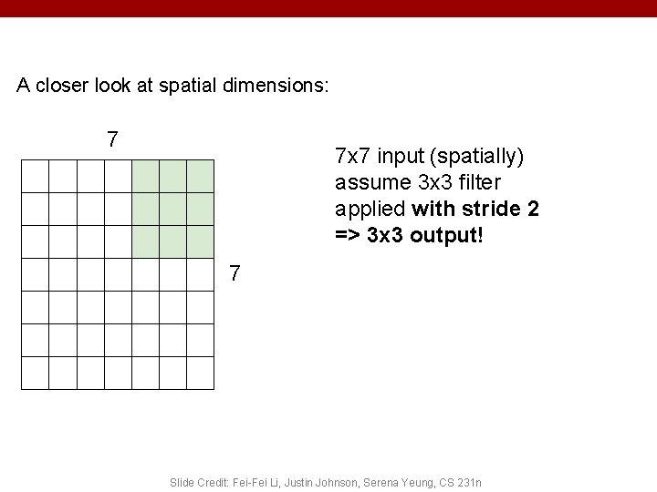
A closer look at spatial dimensions: 7 7 x 7 input (spatially) assume 3 x 3 filter applied with stride 2 => 3 x 3 output! 7 Slide Credit: Fei-Fei Li, Justin Johnson, Serena Yeung, CS 231 n

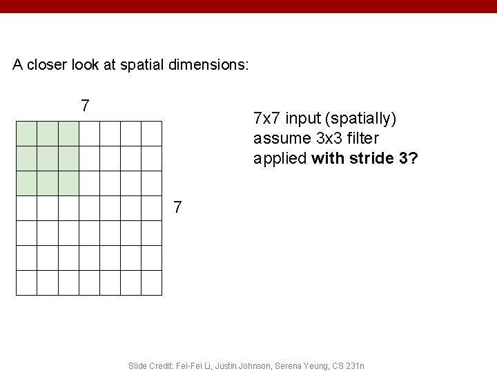
A closer look at spatial dimensions: 7 7 x 7 input (spatially) assume 3 x 3 filter applied with stride 3? 7 Slide Credit: Fei-Fei Li, Justin Johnson, Serena Yeung, CS 231 n

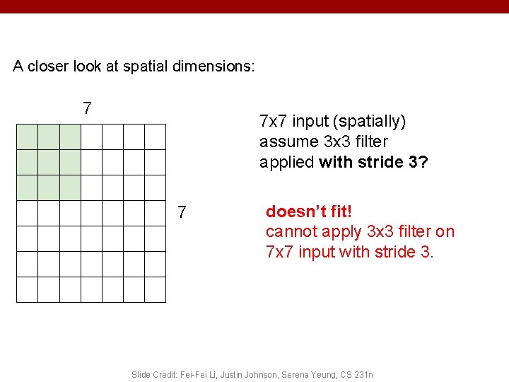
A closer look at spatial dimensions: 7 7 x 7 input (spatially) assume 3 x 3 filter applied with stride 3? 7 doesn’t fit! cannot apply 3 x 3 filter on 7 x 7 input with stride 3. Slide Credit: Fei-Fei Li, Justin Johnson, Serena Yeung, CS 231 n

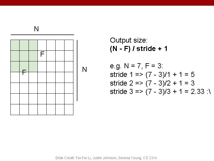
N Output size: (N - F) / stride + 1 F F N e. g. N = 7, F = 3: stride 1 => (7 - 3)/1 + 1 = 5 stride 2 => (7 - 3)/2 + 1 = 3 stride 3 => (7 - 3)/3 + 1 = 2. 33 : Slide Credit: Fei-Fei Li, Justin Johnson, Serena Yeung, CS 231 n

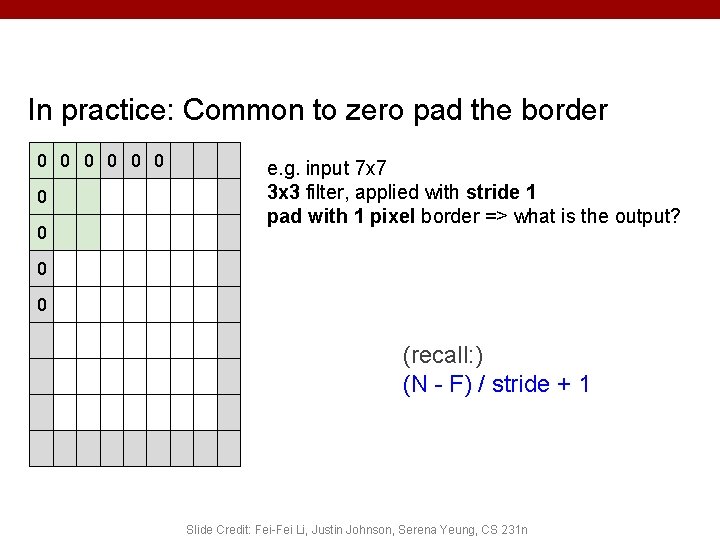
In practice: Common to zero pad the border 0 0 0 0 e. g. input 7 x 7 3 x 3 filter, applied with stride 1 pad with 1 pixel border => what is the output? 0 0 (recall: ) (N - F) / stride + 1 Slide Credit: Fei-Fei Li, Justin Johnson, Serena Yeung, CS 231 n

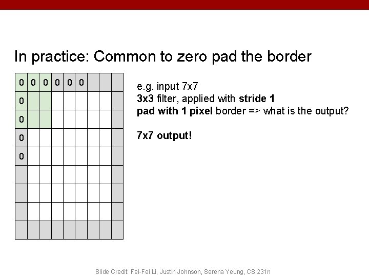
In practice: Common to zero pad the border 0 0 0 0 0 e. g. input 7 x 7 3 x 3 filter, applied with stride 1 pad with 1 pixel border => what is the output? 7 x 7 output! 0 Slide Credit: Fei-Fei Li, Justin Johnson, Serena Yeung, CS 231 n

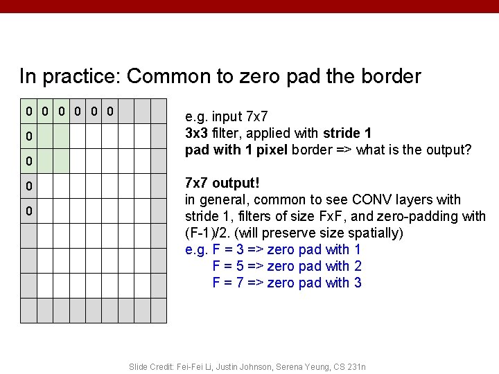
In practice: Common to zero pad the border 0 0 0 0 0 e. g. input 7 x 7 3 x 3 filter, applied with stride 1 pad with 1 pixel border => what is the output? 7 x 7 output! in general, common to see CONV layers with stride 1, filters of size Fx. F, and zero-padding with (F-1)/2. (will preserve size spatially) e. g. F = 3 => zero pad with 1 F = 5 => zero pad with 2 F = 7 => zero pad with 3 Slide Credit: Fei-Fei Li, Justin Johnson, Serena Yeung, CS 231 n

Remember back to… E. g. 32 x 32 input convolved repeatedly with 5 x 5 filters shrinks volumes spatially! (32 -> 28 -> 24. . . ). Shrinking too fast is not good, doesn’t work well. 32 32 3 28 CONV, Re. LU e. g. 6 5 x 5 x 3 filters 28 6 24 CONV, Re. LU e. g. 10 5 x 5 x 6 filters CONV, Re. LU 24 10 Slide Credit: Fei-Fei Li, Justin Johnson, Serena Yeung, CS 231 n ….

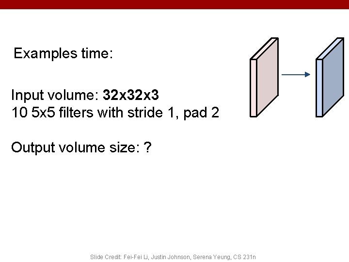
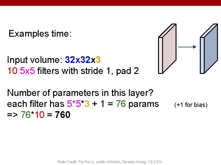
Examples time: Input volume: 32 x 3 10 5 x 5 filters with stride 1, pad 2 Output volume size: ? Slide Credit: Fei-Fei Li, Justin Johnson, Serena Yeung, CS 231 n

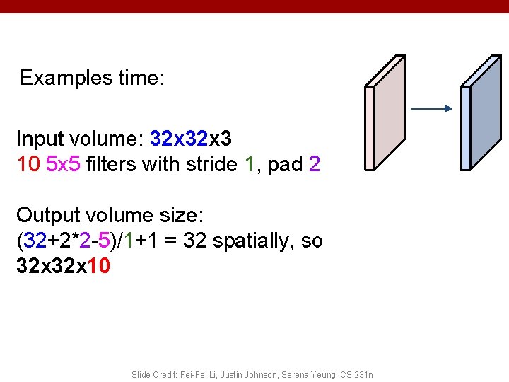
Examples time: Input volume: 32 x 3 10 5 x 5 filters with stride 1, pad 2 Output volume size: (32+2*2 -5)/1+1 = 32 spatially, so 32 x 10 Slide Credit: Fei-Fei Li, Justin Johnson, Serena Yeung, CS 231 n

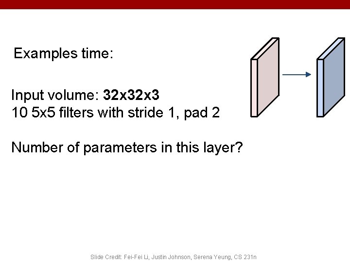
Examples time: Input volume: 32 x 3 10 5 x 5 filters with stride 1, pad 2 Number of parameters in this layer? Slide Credit: Fei-Fei Li, Justin Johnson, Serena Yeung, CS 231 n

Examples time: Input volume: 32 x 3 10 5 x 5 filters with stride 1, pad 2 Number of parameters in this layer? each filter has 5*5*3 + 1 = 76 params => 76*10 = 760 Slide Credit: Fei-Fei Li, Justin Johnson, Serena Yeung, CS 231 n (+1 for bias)

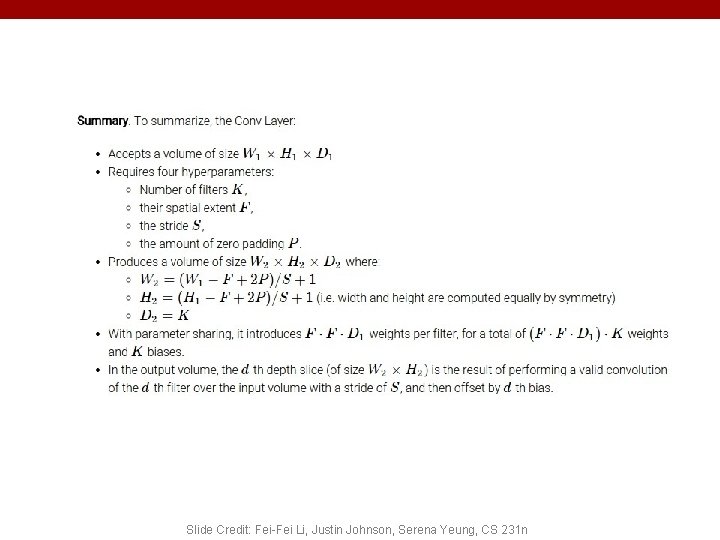
Slide Credit: Fei-Fei Li, Justin Johnson, Serena Yeung, CS 231 n

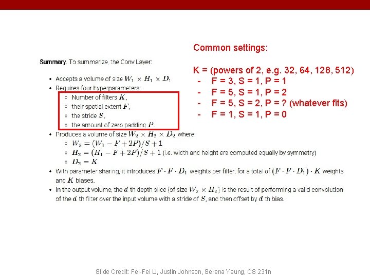
Common settings: K = (powers of 2, e. g. 32, 64, 128, 512) - F = 3, S = 1, P = 1 - F = 5, S = 1, P = 2 - F = 5, S = 2, P = ? (whatever fits) - F = 1, S = 1, P = 0 Slide Credit: Fei-Fei Li, Justin Johnson, Serena Yeung, CS 231 n

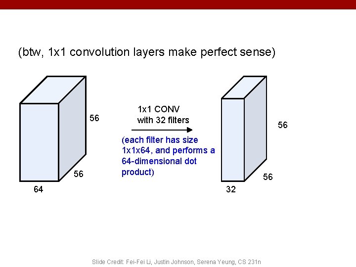
(btw, 1 x 1 convolution layers make perfect sense) 56 56 64 1 x 1 CONV with 32 filters 56 (each filter has size 1 x 1 x 64, and performs a 64 -dimensional dot product) 56 32 Slide Credit: Fei-Fei Li, Justin Johnson, Serena Yeung, CS 231 n

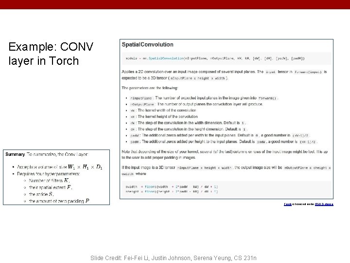
Example: CONV layer in Torch is licensed under BSD 3 -clause. Slide Credit: Fei-Fei Li, Justin Johnson, Serena Yeung, CS 231 n

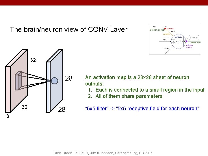
The brain/neuron view of CONV Layer 32 28 32 3 28 An activation map is a 28 x 28 sheet of neuron outputs: 1. Each is connected to a small region in the input 2. All of them share parameters “ 5 x 5 filter” -> “ 5 x 5 receptive field for each neuron” Slide Credit: Fei-Fei Li, Justin Johnson, Serena Yeung, CS 231 n

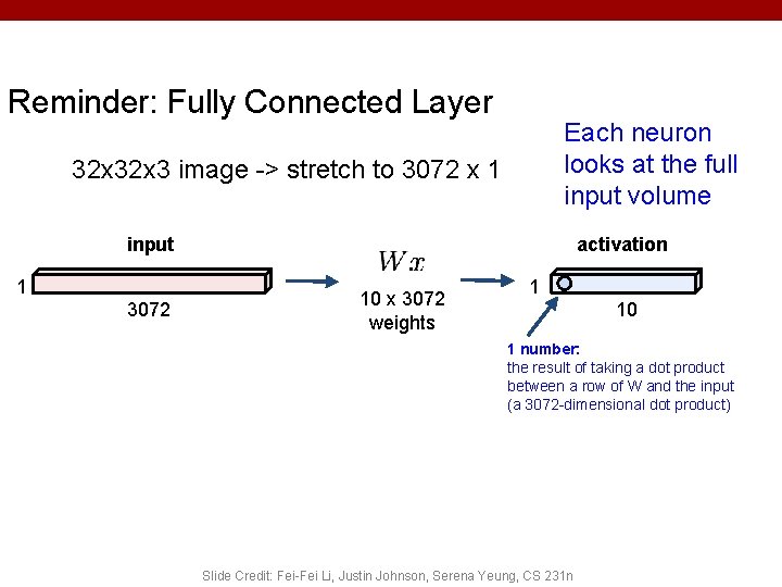
Reminder: Fully Connected Layer Each neuron looks at the full input volume 32 x 3 image -> stretch to 3072 x 1 input 1 3072 activation 10 x 3072 weights 1 10 1 number: the result of taking a dot product between a row of W and the input (a 3072 -dimensional dot product) Slide Credit: Fei-Fei Li, Justin Johnson, Serena Yeung, CS 231 n

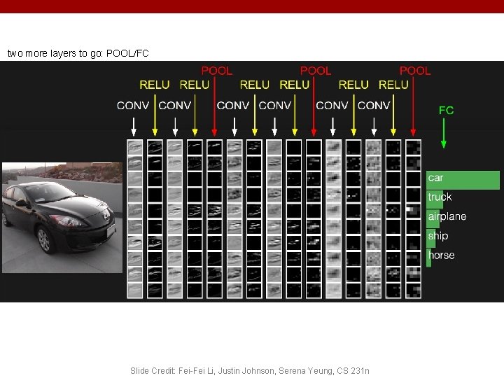
two more layers to go: POOL/FC Slide Credit: Fei-Fei Li, Justin Johnson, Serena Yeung, CS 231 n

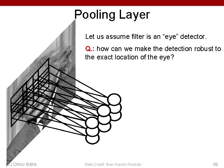
Pooling Layer Let us assume filter is an “eye” detector. Q. : how can we make the detection robust to the exact location of the eye? (C) Dhruv Batra Slide Credit: Marc'Aurelio Ranzato 96

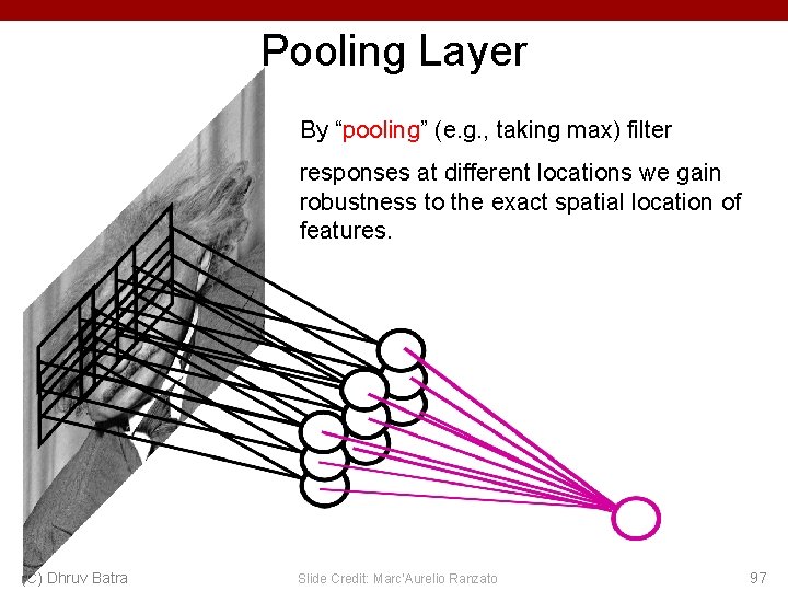
Pooling Layer By “pooling” (e. g. , taking max) filter responses at different locations we gain robustness to the exact spatial location of features. (C) Dhruv Batra Slide Credit: Marc'Aurelio Ranzato 97

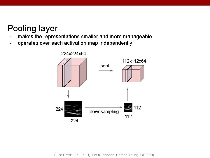
Pooling layer - makes the representations smaller and more manageable operates over each activation map independently: Slide Credit: Fei-Fei Li, Justin Johnson, Serena Yeung, CS 231 n

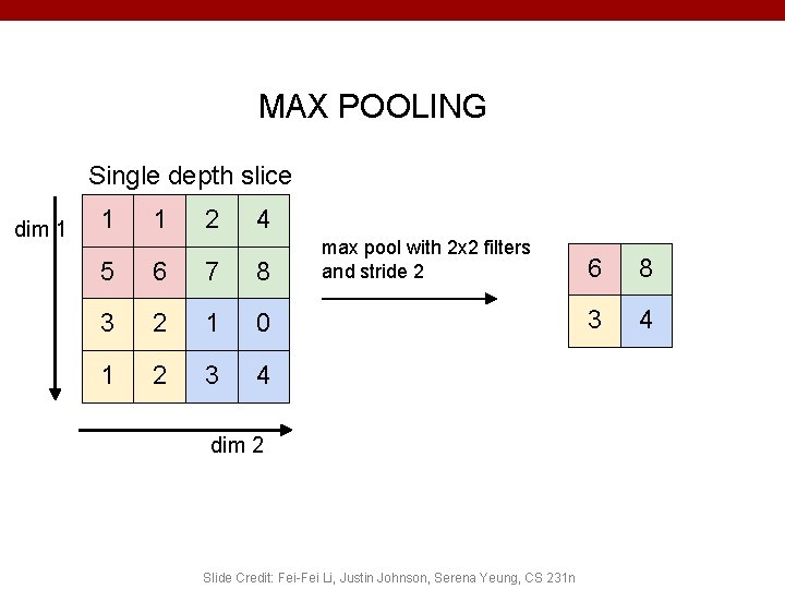
MAX POOLING Single depth slice dim 1 1 1 2 4 5 6 7 8 3 2 1 0 1 2 3 4 max pool with 2 x 2 filters and stride 2 dim 2 Slide Credit: Fei-Fei Li, Justin Johnson, Serena Yeung, CS 231 n 6 8 3 4

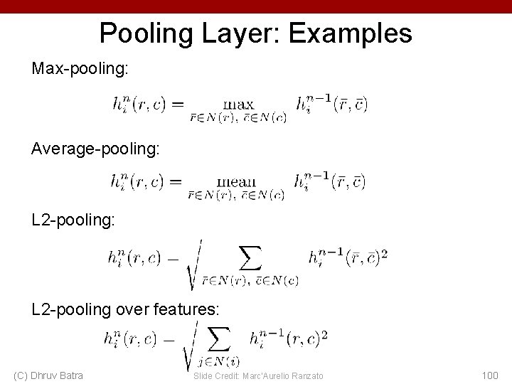
Pooling Layer: Examples Max-pooling: Average-pooling: L 2 -pooling over features: (C) Dhruv Batra Slide Credit: Marc'Aurelio Ranzato 100

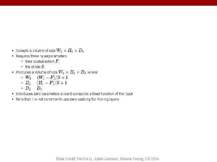
Slide Credit: Fei-Fei Li, Justin Johnson, Serena Yeung, CS 231 n

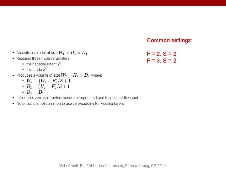
Common settings: F = 2, S = 2 F = 3, S = 2 Slide Credit: Fei-Fei Li, Justin Johnson, Serena Yeung, CS 231 n

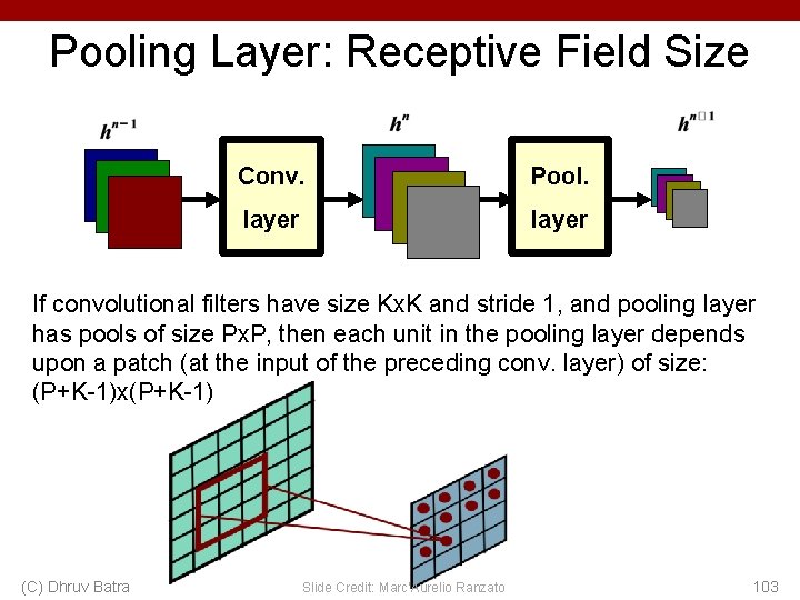
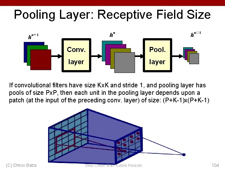
Pooling Layer: Receptive Field Size Conv. Pool. layer If convolutional filters have size Kx. K and stride 1, and pooling layer has pools of size Px. P, then each unit in the pooling layer depends upon a patch (at the input of the preceding conv. layer) of size: (P+K-1)x(P+K-1) (C) Dhruv Batra Slide Credit: Marc'Aurelio Ranzato 103

Pooling Layer: Receptive Field Size Conv. Pool. layer If convolutional filters have size Kx. K and stride 1, and pooling layer has pools of size Px. P, then each unit in the pooling layer depends upon a patch (at the input of the preceding conv. layer) of size: (P+K-1)x(P+K-1) (C) Dhruv Batra Slide Credit: Marc'Aurelio Ranzato 104

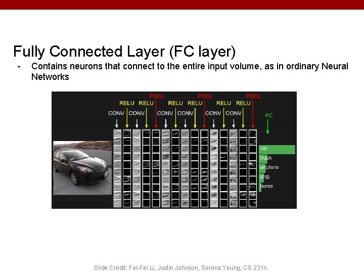
Fully Connected Layer (FC layer) - Contains neurons that connect to the entire input volume, as in ordinary Neural Networks Slide Credit: Fei-Fei Li, Justin Johnson, Serena Yeung, CS 231 n

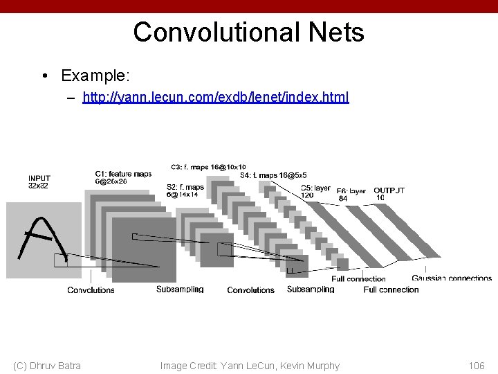
Convolutional Nets • Example: – http: //yann. lecun. com/exdb/lenet/index. html (C) Dhruv Batra Image Credit: Yann Le. Cun, Kevin Murphy 106

Classical View (C) Dhruv Batra Figure Credit: [Long, Shelhamer, Darrell CVPR 15] 108

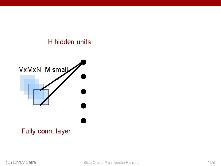
H hidden units Mx. N, M small Fully conn. layer (C) Dhruv Batra Slide Credit: Marc'Aurelio Ranzato 109

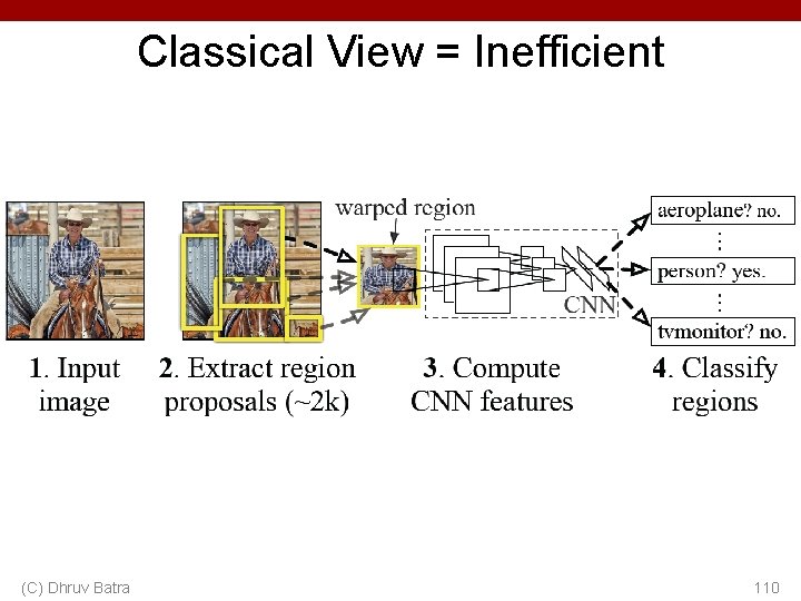
Classical View = Inefficient (C) Dhruv Batra 110

Classical View (C) Dhruv Batra Figure Credit: [Long, Shelhamer, Darrell CVPR 15] 111

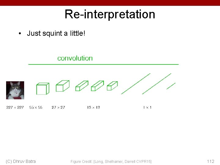
Re-interpretation • Just squint a little! (C) Dhruv Batra Figure Credit: [Long, Shelhamer, Darrell CVPR 15] 112

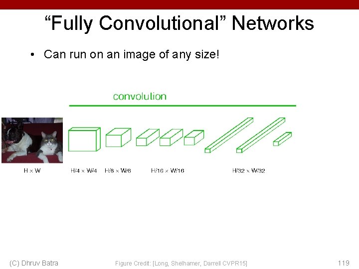
“Fully Convolutional” Networks • Can run on an image of any size! (C) Dhruv Batra Figure Credit: [Long, Shelhamer, Darrell CVPR 15] 113

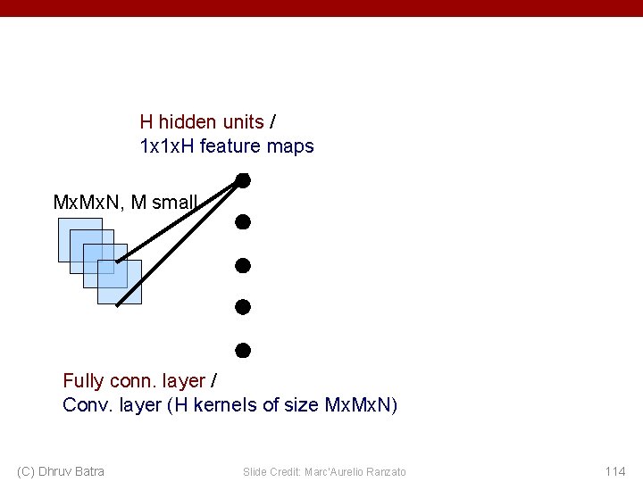
H hidden units / 1 x 1 x. H feature maps Mx. N, M small Fully conn. layer / Conv. layer (H kernels of size Mx. N) (C) Dhruv Batra Slide Credit: Marc'Aurelio Ranzato 114

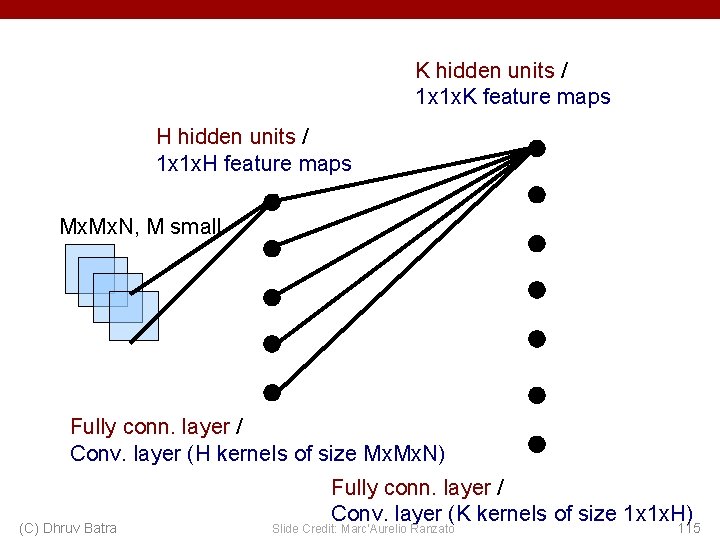
K hidden units / 1 x 1 x. K feature maps H hidden units / 1 x 1 x. H feature maps Mx. N, M small Fully conn. layer / Conv. layer (H kernels of size Mx. N) (C) Dhruv Batra Fully conn. layer / Conv. layer (K kernels of size 1 x 1 x. H) Slide Credit: Marc'Aurelio Ranzato 115

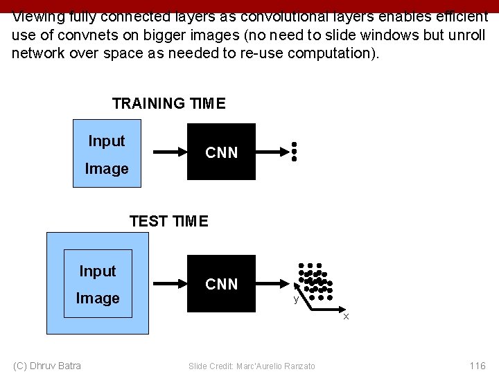
Viewing fully connected layers as convolutional layers enables efficient use of convnets on bigger images (no need to slide windows but unroll network over space as needed to re-use computation). TRAINING TIME Input Image CNN TEST TIME Input Image CNN y x (C) Dhruv Batra Slide Credit: Marc'Aurelio Ranzato 116

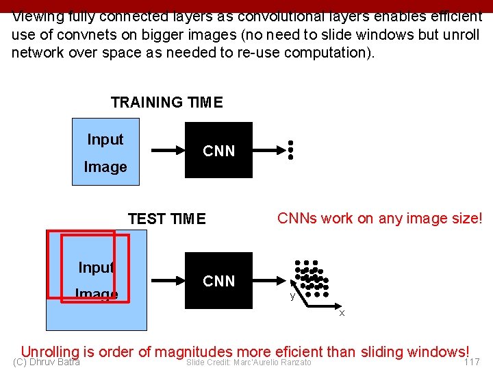
Viewing fully connected layers as convolutional layers enables efficient use of convnets on bigger images (no need to slide windows but unroll network over space as needed to re-use computation). TRAINING TIME Input Image CNN TEST TIME Input Image CNNs work on any image size! y x Unrolling is order of magnitudes more eficient than sliding windows! (C) Dhruv Batra Slide Credit: Marc'Aurelio Ranzato 117

Re-interpretation • Just squint a little! (C) Dhruv Batra Figure Credit: [Long, Shelhamer, Darrell CVPR 15] 118

“Fully Convolutional” Networks • Can run on an image of any size! (C) Dhruv Batra Figure Credit: [Long, Shelhamer, Darrell CVPR 15] 119

Benefit of this thinking • Mathematically elegant • Efficiency – Can run network on arbitrary image – Without multiple crops (C) Dhruv Batra 121

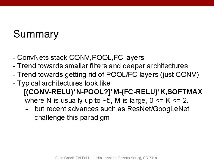
Summary - Conv. Nets stack CONV, POOL, FC layers - Trend towards smaller filters and deeper architectures - Trend towards getting rid of POOL/FC layers (just CONV) - Typical architectures look like [(CONV-RELU)*N-POOL? ]*M-(FC-RELU)*K, SOFTMAX where N is usually up to ~5, M is large, 0 <= K <= 2. - but recent advances such as Res. Net/Goog. Le. Net challenge this paradigm Slide Credit: Fei-Fei Li, Justin Johnson, Serena Yeung, CS 231 n